
Resonance, Pulsing, Gradients, and Weights
Objectives:
- Define resonance and give examples of various types of resonance
- Define Larmor’s frequency
- Explain how field strength affects the frequency of hydrogen protons
- Define TE and TR
- Explain T1, T2 and T2*
- Explain a spin echo
- Differentiate between the longitudinal component and transverse component of the magnetization vector.
- Differentiate between the 90-degree and 180-degree RF pulse and explain why each is used.
- Define the sinusoidal wave
- Explain T2 decay
- Define and explain gradients
- List the three gradients used in MR Imaging
- Explain how Larmor’s frequency relates to the use of gradients
- Define which parameters control T1 weighting
- Define which parameters control T2 weighting
- List the weighting values and appearance of tissue on a T1 and T2 sequence
- List the impact on the signal of the various parameters used in T1 and T2 sequences
- Describe how contrast agents affect tissue weighting
- Define and differentiate between TE and TR
- Define SNR
Description:
This article introduces the learner to the concept of resonance, where we will discuss the magnetization vectors, both Macro and Micro, which occur at the nuclear level, we will dive into some basic pulse sequence information. Also, we will discuss gradients and how they are used to define where, in a given space, the resonance and signal will occur. Lastly, we are going to concentrate on the various weighting of tissues in the body. We will also learn the basics of how to adjust the TE and TR to control how tissue appears on the MR image, what these different contrasts to tissue look like and the impact on the signal as we make adjustments to TE and TR for contrast. This article is accredited by the ASRT for 1.75 Category A CE Credits.
This article introduces the learner to the concept of resonance. We will also discuss the magnetization vectors, both Macro and Micro, which occur at the nuclear level. We will dive into some basic pulse sequence information, a topic we will discuss in greater detail in subsequent lessons, but one we need to understand in order to understand how the signal is created. Lastly we will discuss gradients and how they are used to define where, in a given space, the resonance and signal will occur.
Resonance
Resonance refers to the transfer of energy between two oscillating systems, provided they are oscillating at the same frequency.
Definition
Resonance means the Transfer of energy between two systems that oscillate at the same frequency. This definition of resonance is essential to understand the function of MRI. It will allow us to understand the principle of radiofrequency pulses or even the operation of gradients.
Examples of Resonances
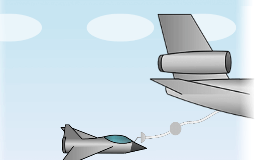
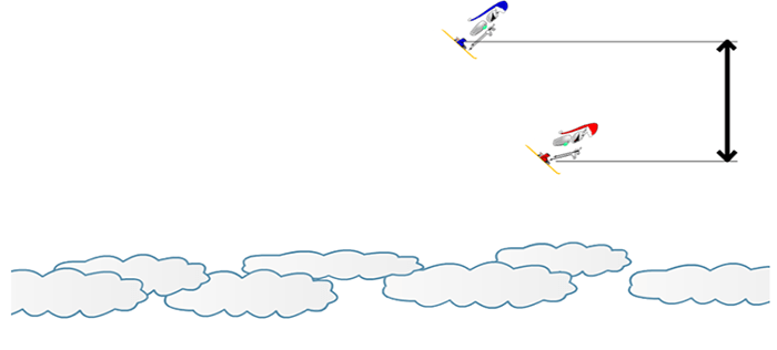
In order for a tanker to transfer energy in the form of fuel to a small plane, both must be flying at the same speed, otherwise, energy transfer is impossible.
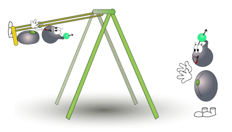
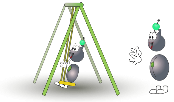
This is an example of genuine resonance. The first system is the swing. Its frequency is always the same, in other words, the swing will always take the same time to go from one maximum to the second. The higher the velocity, the higher the maximum. The second system is the arm of the person pushing it. Very young, we instinctively learn that to transfer energy to the swing, we have to push at a precise frequency which is that of the swing itself. In this case, energy is transferred from the arm of the person pushing to the swing which is thus accelerated.
Every material has its own resonance frequency. That of crystal glass is within the frequency range that humans can receive and transmit. This explains, in theory at least, why a diva can make the crystal glass vibrate in resonance with her voice and shatter it by the induced vibrations.
In reality, the frequency emitted must be pure and have a very narrow bandwidth. The human voice emits sounds over a broad bandwidth. The emitted energy is thus dispersed and is not concentrated enough to make the crystal vibrate to the breaking point. No person has yet been able to produce this sound. When an earthquake occurs, the ground vibrates with a given frequency. If this frequency is the same as the resonance frequency of the building, it resonates with the seismic waves and starts rocking until it collapses.
Larmor’s Frequency
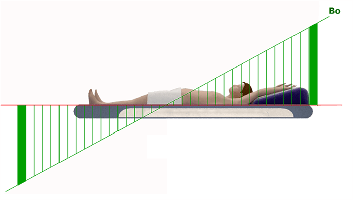
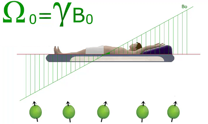
Larmors’ mathematical formula is one of the rare formulas that must be known in MRI. It shows simply that the rotation velocity (W0) of protons placed in a magnetic field depends on the nature of the nucleus in question, characterized by a gyromagnetic constant Gamma γ (dependent on the type of nucleus), and also on the intensity of the magnetic field B0.
Thus, the stronger the field, the higher the rotation velocity of protons. One Hertz is one rotation per second and so the velocity of a hydrogen proton in a 1.5 T magnetic field is 63.8 million rotations per second.
Examples of Frequencies
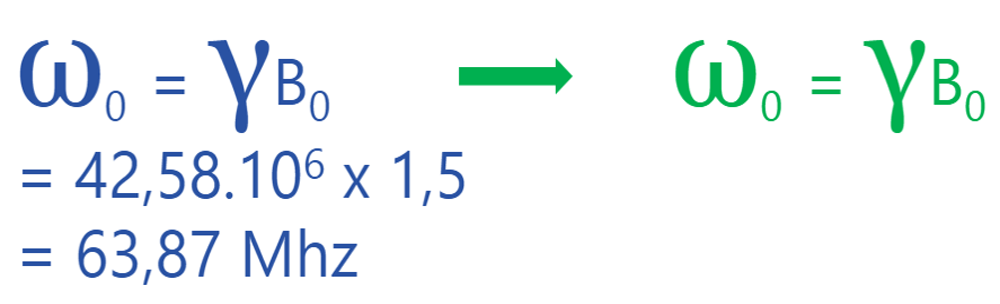
We have seen that the rotation velocity of a proton depends on the intensity of the magnetic field. At 1 Tesla, the hydrogen protons resonate at 42.58 MHz. To find the resonance of the hydrogen proton in other field strengths, we simply multiply 42.58 times the strength of the magnet. The most common field strength used in MRI is 1.5T. Therefore, the resonance of the hydrogen proton in a 1.5T scanner would be 1.5 X 42.58 or 63.87MHz as is shown here. Note that in a 3T scanner it is much faster!!
Classification
| Field B0(t) for Hydrogen proton | Larmor frequency (MHz) |
| 0.35 | 14.90 |
| 1 | 42.58 |
| 1.5 | 63.87 |
| 3 | 127.74 |
This table shows the classes of different waves with respect to their inherent frequencies. We can see that the rotation frequency of the hydrogen proton is in the range of radio frequencies.
Note that Xrays have very high frequencies, greater than 3000 THz, and on the other end of the spectrum, terrestrial magnetic fields are at 0 Hz. The frequencies that can make a hydrogen proton resonate are in the range of radiofrequency (RF) waves. This range is 30 kHz to 300 GHz.
| Electromagnetic wave | Frequency | Application |
| X-Ray | > 3000 THz | Medical imaging radiography |
| UV Ray | 750 THz to 3000 THz | Solar light |
| Visible color | 385 THz to 750 THz | Human vision, Photosynthesis |
| Infrared | 0.3 THz to 385 THz | Warm |
| Radiofrequency wave | 30 KHz to 300 GHz | Television, FM Radio |
| Very low frequency (VLF) | 3 KHz to 30 KHz | Radio-communications |
| Audio frequency (AF) | 0.3 KHz to 3 KHz | Trasnmission of vocal datas |
| Terrestral magnetic field | 0 Hz | Indicate the north |
Magnetization is something that will occur naturally when anything that has magnetic potential is introduced to the large magnet. Let’s learn a little more about what is meant by the magnetization vector and describe this magnetization that occurs during an MRI procedure.
Definition
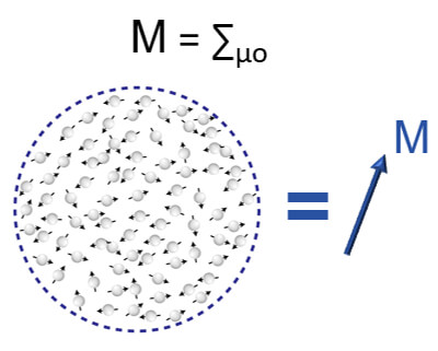
In MRI we have microscopic magnetization vectors in the form of the individual spinning protons. We also have a macroscopic magnetization vector which is the SUM of ALL microscopic magnetization vectors. This macroscopic magnetization is represented by the formula shown here. In other words, the macroscopic magnetization vector is equal to the total sum.
So, how do we create a magnetic field? If we place a permanent magnet on a surface coated with iron filings we can easily see the field lines on both sides of the magnet. Because of the ferrous properties of the iron filings, they are naturally attracted to the magnet. The Iron fillings with gather around and attach to the magnet within these field lines. Even if they do not all attach directly onto the magnet, they are within the magnetic field.
Macroscopic Magnetization Vector
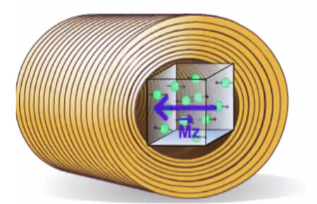
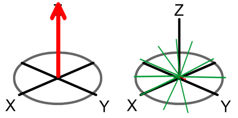
We saw that a hydrogen atom can be compared to a small rotating dipole, shown by a macroscopic magnetization vector. This is what we see at the beginning of the animation. Our bodies are obviously not composed of a single hydrogen atom, which is why we will see what happens at the macroscopic level: the macroscopic magnetization vector is the sum of all the minute microscopic magnetization vectors.
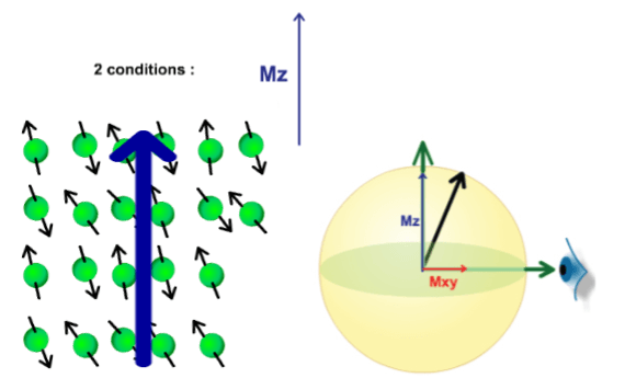
This macroscopic magnetization vector is, in fact, the resultant of two components: the component along the longitudinal axis Mz and the component along the transverse plane Mxy. In order to better understand the notions that will follow, we will distinguish each of these components. Something happens on the longitudinal axis that affects component Mz and at the same time, something happens on the transverse plane that affects component Mxy.
The Longitudinal Component
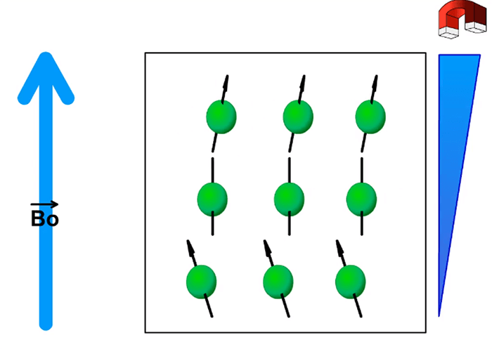
We now see the sum of all microscopic magnetization vectors along Mz. If spins are not aligned the sum of all the small vectors will be zero. If spins are all aligned but half are oriented in one direction and the other half in the opposite directions, the sum of all these small magnetization vectors is still zero.
We need to have an odd number aligned in one direction or the other. In order to have a longitudinal component Mz, two conditions must be fulfilled:
- Protons are aligned on the same direction
- There is an excess of protons in one direction compared to the other
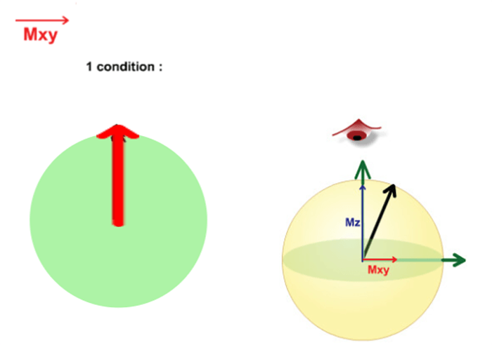
The Transverse Component
If spins are not in phase, they are distributed all around the precession cone and the sum of all these vectors is zero. This is why all protons must be in phase in order to have a transverse component Mxy.
In this next section, we will discuss basic MRI pulse sequences, what they look like chronologically along with what happens to the spinning protons during pulse sequences. It is important in MRI to understand what is happening to the protons, to fully understand how to create the best images possible. Slight changes in parameters (which we will learn more about as we go) can have a dramatic effect on what is seen in the final image.
Chronology
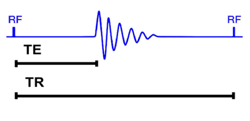
When an MRI sequence is reduced to its simplest expression: the repetition of a 90° radiofrequency pulse followed by gathering information in the form of a signal. The symbol RF demonstrates the application of the radiofrequency. The sinusoidal wave represents the signal given off by the proton while T1 and T2 relaxation are occurring.
With this sequence, we introduce the notion of TE and TR. TE: the time from initiation of the RF pulse and the time the echo is collected. This is called Time to Echo or TE for short. TR: the time after which the basic pattern of the sequence is repeated. The basic pattern here is a 90° pulse followed by signal collection, then followed by another 90 degree RF pulse. TR stands for Time to repetition.
Notice how after initial RF energy is applied, the signal is first strong, characterized by the high amplitude of the wave, and then it slowly declines to the point where it is no longer giving a signal. This is important because we want to try to collect the echo as close to the stronger end of the signal as possible.
Reminder: Identical Frequencies
The systems must oscillate at the same frequency. We saw that the frequency of a hydrogen proton in a 1.5 T field strength is 63.87 MHz. A radio frequency wave of 63.87 MHz must thus be emitted in order to make these protons resonate. Remember, if both systems are not operating at the same frequency, nothing will happen. No energy is transferred.
Protons in B0 Field
What happens at the level of the macroscopic magnetization vector by differentiating component Mz and component Mxy?
When protons are outside the magnetic field, they are not aligned along the main direction: component Mz of the macroscopic magnetization vector is thus null. Also, protons are not in phase: component Mxy of the macroscopic magnetization vector is also null. In summary, the macroscopic magnetization vector is zero.
This happens when protons are subjected to the magnetic field, B0. They are now aligned along the main axis of B0 and a slight excess of protons are oriented parallel to field B0 compared to that oriented antiparallel to B0: the two conditions for having a component Mz are thus fulfilled. Furthermore, the protons are still not in phase: component Mxy of the macroscopic magnetization vector is thus still zero. The macroscopic magnetization vector has been reduced simply to its longitudinal component Mz.
Mz in Detail
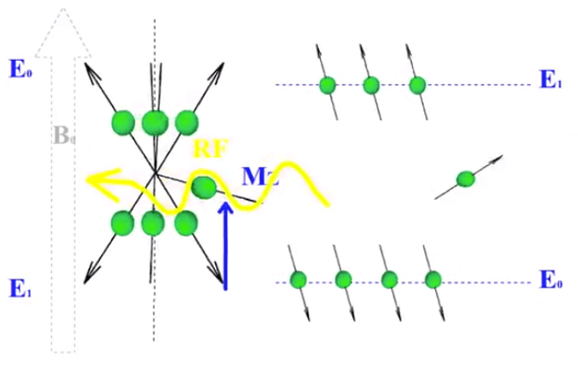
In steady-state or “resting” state, the conditions for having a component Mz are fulfilled: protons are aligned along the axis of B0 with excess protons in the parallel direction compared to the antiparallel direction. If we show this from an energy standpoint, the parallel direction is low energy and the antiparallel direction is high energy: there are thus more low energy protons than high energy protons.
When the radio frequency wave is applied, protons start resonating and will receive energy transmitted by the wave. When low energy protons absorb this energy they will be shifted to high energy levels. This will equalize the populations of low and high energy protons. This causes the second condition for having component Mz to disappear, and so Mz is null.
Mxy in Detail
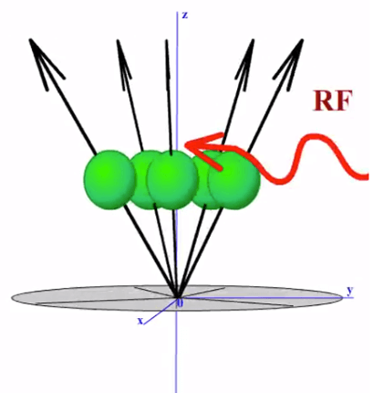
In order to understand what happens at the level of component Mxy, we will concentrate only on the positive part. If we regard the projection of all these microscopic magnetization vectors in the transverse plane, protons are not in phase and so the sum of these vectors is zero: there is no transverse component in steady-state. When the radio frequency wave is applied, resonance causes the different spins to enter in phase: a transverse component is created.
The pulse of 90°
When the radio frequency wave is applied, two things happen:
- Equalization of populations of protons parallel to B0 and protons antiparallel to B0, causing the disappearance of component Mz
- Different spins are created that leads to the appearance of component Mxy
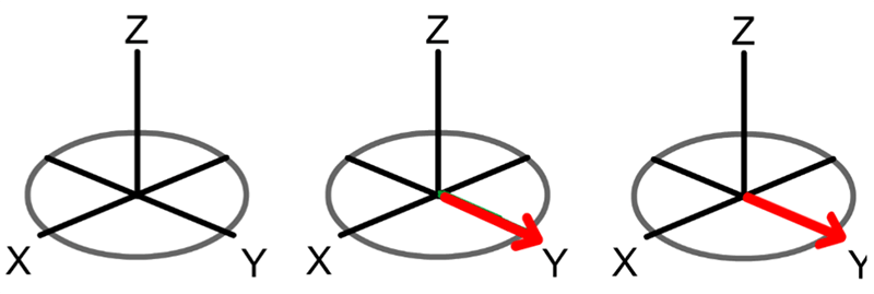
The macroscopic magnetization vector (M) is reduced to simply its transverse component Mxy. Starting from the steady-state where this magnetization vector was reduced simply to its longitudinal component Mz, we have flipped this macroscopic magnetization vector 90°. Common language usage talks about flipping protons but in reality, what has been flipped is the macroscopic magnetization vector because of the phenomenon occurring in the longitudinal axis and another that occurs in the transverse plane.
Relaxations
After the 90° pulse, protons return to their steady-state:
- Excess protons oriented in the parallel direction progressively return and the longitudinal component Mz also progressively returns. This is T1 relaxation or longitudinal relaxation
- The protons progressively de-phase, and the transverse component Mxy progressively decreases. This is T2 relaxation or transverse relaxation
These relaxations take place at the same time but not at the same rate. T2 relaxation is much more rapid. In order to facilitate understanding, we can accept to say that it occurs before T1 relaxation. Furthermore, these relaxations are not linear over time.
T1 Relaxation
At the end of the 90° pulse, the longitudinal component is null, after which it will gradually increase. This increase is not linear: very rapid at the start, its rate decreases until reaching a maximum, the steady-state. This means that the return of excess protons oriented parallel to B0 was rapid at first and then became slower and slower. Everybody tissue has its own rate of T1 relaxation in order to differentiate tissues. All tissue must be assigned their own T1 value. The T1 of a tissue is the time necessary for this tissue to reach 63% of its T1 relaxation.
T2 Relaxation
At the end of the 90° pulse, the transverse component is maximum, after which it gradually decreases. This decrease is not linear: it is also very rapid at the start, its rate progressively decreases, tending toward zero, the steady-state. This means that spin de-phasing is rapid at the start and the rate then gradually decreases.
Everybody tissue has its own rate of T2 relaxation. In order to differentiate tissues, we assign them their own T2 value. The T2 of a tissue is the time necessary for this tissue to reach 63% of its T2 relaxation, in other words, the time after which there remains 37% of transverse magnetization.
Definition
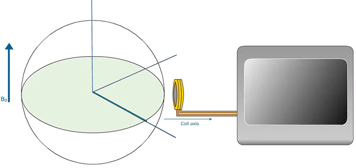
Again, the signal is the echo given off of the protons during T1 and T2 relaxation. It is very similar to the concept that of Ultrasound. In MRI, the coil is the communication tool between the protons of the patient and the system. It reflects small changes in the magnetic field detected in the patient’s electrical signal. The signal is recorded as a sine curve. As with any sine curve, the frequency will be the same, but the amplitude, which signifies the intensity can be different. The signal can be detected in the plane transverse to B0.
We detect very small changes in the magnetic field however the primary goal is to be able to collect these small variations in the direction of B0. It is for this reason that the coil design must be adapted to the direction of the main field. Thus, a coil designed for a vertical field magnet cannot be used for a horizontal field because B0 is obviously on a different plane.
Sinusoïd
The signal is a sine curve because of the fact that protons rotate. When they pass in front of the antenna detector, the signal is maximum. When they are on the opposite side of the circle described by their precession cone, the signal is minimal
In our metaphor, Hydro is sitting on a chair, emitting a constant sound. When he is facing us we hear a sound at the maximum of its intensity. When he has his back to us, sound intensity is minimal. If we show signal intensity, or the sound heard from Hydro over time, we obtain a sine curve.
Decreasing Sinusoïd
The signal recorded in MRI is decreasing since there is the dispersion of the signal, resulting from spin dephasing. At the end of the radiofrequency pulse, the signal is maximum because all protons are in phase and so pass in front of the antenna detectors at the same time. Spins will then gradually dephase and disperse around the precession cone. The signal will become diluted.
If we extend the previous metaphor, Hydro is no longer sitting on a chair, but there is a choir of Hydros on a merry-go-round. If the Hydros are close to one another (in-phase) the sound we hear is maximum. If they are now dispersed around the periphery of the merry-go-round, the sound is more diluted and thus weaker.
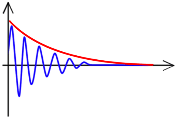
F.I.D
As mentioned earlier, as time passes, the signal will decrease – this is because once the protons relax back to align with the magnetic field, they are no longer giving off a signal or echo.
If we plot a curve joining the waves of this decreasing sine curve, the shape we obtain is already familiar: This is T2 decay. This is a good thing since the signal is captured in the transverse plane and T2 decay corresponds to transverse relaxation. This decay is called FID (Free Induction Decay).
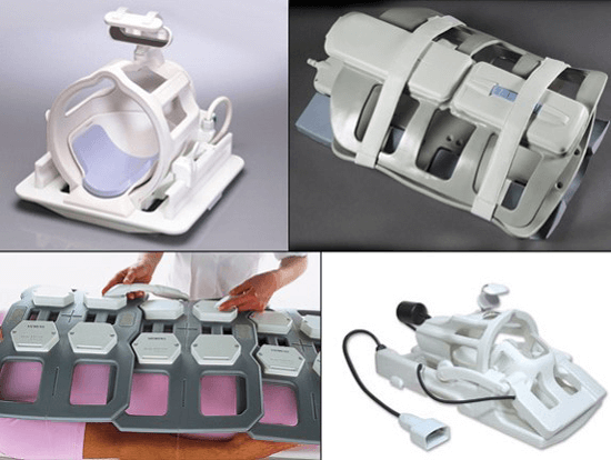
The Coils
In order to create an image of the signals given off during this process, we need an antenna. In MRI, this antenna is called a coil. The coil works in the same way as an antenna on a car to pick up radio stations, or a TV antenna if you remember what that is. Television and radio, use radio waves to transmit information – the antenna picks it up and converts it to sound or a picture. Another way to state this is that the antenna acts as the communication tool between the radiowaves and your TV or radio.
Similarly, The coil is the communication tool between the protons of the patient and the system. It reflects small changes in the magnetic field detected in the patient’s electrical waves. The signal is damped sine shape. The signal can be detected in the plane transverse to B0. Again we are able to detect very small changes in the magnetic field and the primary to be able to collect these small variations in the direction of B0. It is for this reason that the coil design must be adapted to the direction of the main field. Thus, a coil designed for a vertical field cannot be used for a horizontal field.
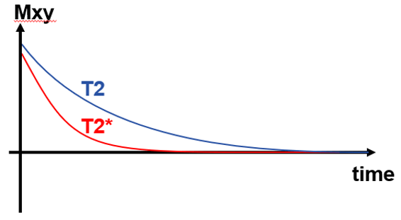
T2* Decay
We saw previously that FID decreased according to T2 decay. In reality, things are a bit more complicated than that. Although the field used in MRI is very homogeneous from a macroscopic standpoint, the same is not true at the microscopic level where there are many local magnetic field inhomogeneities.
As a result of these local inhomogeneities, spins will dephase much more rapidly than if they obeyed T2 decay. The decrease observed is much more rapid. The signal, in fact, decreases according to what is called T2* decay. In order to detect a signal detected according to a T2 decay, we use a sequence called spin echo. This sequence is the basis of MRI and we will now explain its principle.
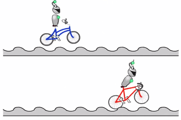
Inhomogeneities
If the road is smooth or homogeneous, the distance between the slow and fast rider increases gradually they dephase according to T2. The distance between them increases more rapidly they dephase according to T2*. The inhomogeneities accelerate the phase shift.
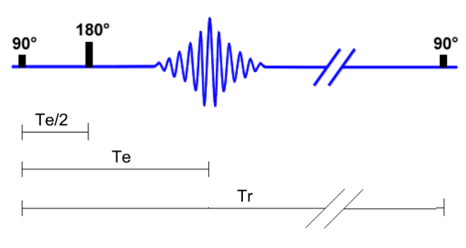
Spin Echo: Chronogram
The spin-echo sequence is characterized by a 180° pulse we will inject between the first radio frequency pulse and signal recovery. This 180° pulse will be applied precisely at time TE/2 or 1/2 of one TE.
This 180° pulse will enable us to get rid of dephasing resulting from the inhomogeneities of magnetic fields and thus rise along the T2 decay curve. The spin-echo sequence is thus the repetition of a 90° pulse, a 180° pulse at TE/2 and signal recovery at TE. This cycle starts again after time TR.
The 180° Pulse
The 180° pulse allows us to get rid of the local magnetic field inhomogeneities. At the end of the 90° pulse, protons are in phase. Spins have had the time of dephasing and we apply a 180° refocusing pulse. The protons continue to rotate in the same direction. If we wait for the same period, the protons are once again in phase. This is the moment when we record the signal. In practice, we select the signal recovery time and the system automatically positions the 180° pulse at time TE/2.
T2 Decay
This 180° flip enables us to get rid of the dephasing caused by local magnetic field inhomogeneities, but not that caused by T2 decay. This is why we can rise along the curve but not all the way to the starting point. Because of the 180° pulse, the signal increase back to the curve then decreases again according to the T2* decay.
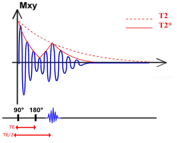
In this case, we see an FID (T2* decay) as early as the end of the 90° pulse followed by a rephasing until the T2 curve is again followed by a T2* decay.
Do you know what happens when we try to touch two magnets together? They repel each other. Gradients are used in a similar way. Gradients are applied to provide localization of the area of protons being effected by the RF signal and ultimately collected by the coil.
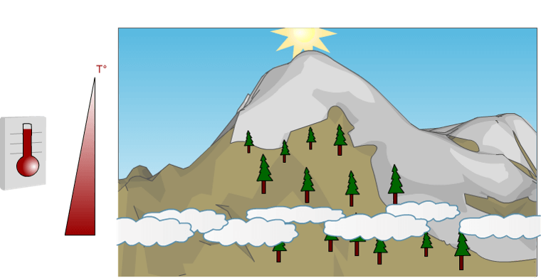
Definition and Examples
A basic definition of a gradient is a variation of physical size in space when looking at the visual representation of a gradient – as a slope. Here the visual gradient represents a warmer temperature at the bottom of the mountain and lower temperature at the top. There are unlimited examples of gradients. Here we can see that increasing altitude leads to decreasing temperatures: there is thus a temperature gradient from top to bottom.
Here is another example: The beach. The further we are from the shoreline, the deeper the water: there is a depth gradient as a function of distance from the shore. What is interesting, in this example is the induced gradient. The greater the depth, the higher the pressure. There is thus a pressure gradient induced by the depth gradient.
In MRI a magnetic gradient will induce a gradient of proton rotation velocity since the rotation velocity of protons depends on the value of the magnetic field: We call this Larmor’s formula.

Specificities and Applications
Gradients are used in MRI to provide Linear and symmetrical modification of the main field, that can be turned on and off very quickly, producing a characteristic sound on running machines. So all of those banging noises you hear in MRI are the gradients at work. As a side note, the stronger the gradients, the louder the scanner. Though many vendors have special configurations to try to quiet the gradients as much as possible. BUT, no matter how much it bothers us or the patients, gradients are essential in MRI.
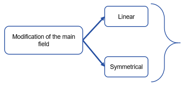
Linear and Symmetrical Gradient
- Linear: This change will create a linear variation of the main field
- Symmetric:this variation is symmetrical on both sides of the center of the magnet in any direction in which it is applied
Modification of the magnetic field creates a linear magnetic field gradient. This means that the magnetic field varies by the same intensity for each unit of distance in the direction in which the gradient is applied. This gradient is also symmetrical. This means that magnetic field variations on both sides of the center of the volume are of the same intensity and have opposite signs for equal distances in the direction in which the gradient is applied.
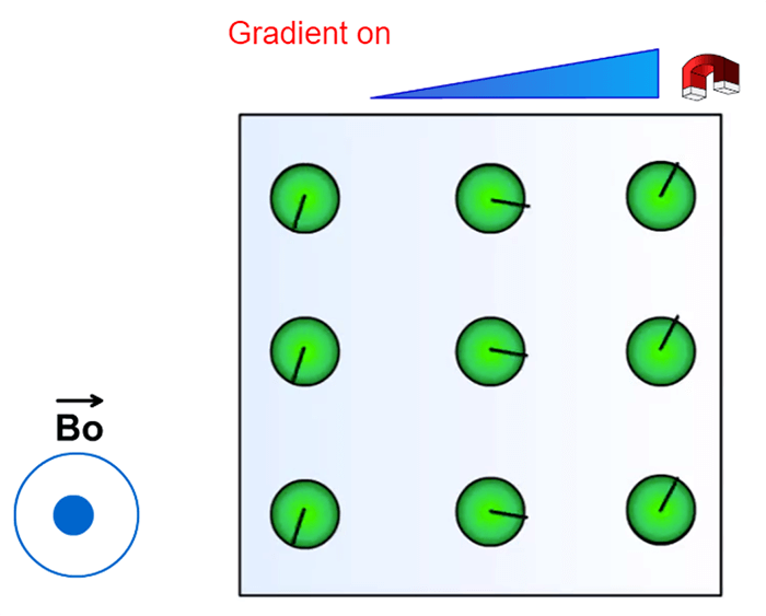
Larmor Frequency
As proton spin speed depends on magnetic field strength, the creation of a magnetic field gradient also gives rise to a proton spin speed gradient. According to Larmor’s formula, the spin speed of protons subjected to a magnetic field is directly proportional to magnetic field strength. This implies that if two identical protons are subjected to different magnetic field strengths, they will have different spin speeds.
These properties are used to:
- Select a slice
- Mutually de-phase protons
- Localize protons according to their spin speed
This is why we give different names to the different gradients used. They are slice selection, phase, and frequency. But it must be borne in mind that it is the same thing every time: a magnetic field gradient that generates a proton spin speed gradient since proton spin speed depends on the value of the magnetic field.
Application of Gradient
When we say a magnetic field gradient, we say the speed of rotation gradient. As we have just seen, if protons are subjected to the same magnetic field, they will have the same frequency. If we now apply a magnetic field gradient, they are no longer subjected to the same field strength and will have different frequencies.
Types of Gradients Used in MRI
In MRI there are three gradients:
- The Slice Selection Gradient (Gss) which moved along the magnetic field or determines the location of the slice along the z-axis of the patient
- The Phase Gradient (Gφ)
- The Frequency Gradient (Gf)
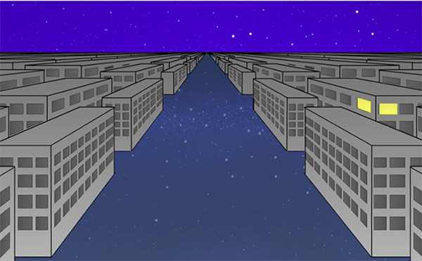
The metaphor of the City
These gradients determine the location in the X or Y direction. Phase can run in x or y and frequency can run X or Y direction. This is something we determine in our parameters and protocol. The 3 gradients allow us to locate the right apartment.
We have here an American city with its perpendicular streets and avenues. The first gradient, called section selection is used, as its name suggests, to intensify a given section. The phase gradient enables us to select an avenue for this floor and finally, the frequency gradient enables us to select a street for this floor and avenue. We have thus isolated a single apartment that is identified in 3 dimensions.
Slice Selection Gradient
The most important thing to remember is that even though we give MRI gradients different names (section selection, phase, and frequency), they are all identical. They are linear and symmetrical magnetic field gradients that involve linear and symmetrical gradients of proton rotation velocity.
We know that in order for resonance to occur, the proton rotation velocity must be equal to the frequency of the emitted wave. The section selection gradient is thus applied at the same time as the radio frequency wave. Only protons whose frequency is equal to that of the emitted wave will start resonating. The others rotate too rapidly or too slowly to resonate with the radio frequency wave.
The Phase Gradient
Each line is subject to a different intensity field, their protons turn at their own different speed: they will dephase. Thus, the Phase Gradient differentiates the different lines according to their phase. Example: We have now isolated one section (or one floor if we take the city metaphor). We now have to sort the signal with respect to its phase and frequency (street and avenue).
A second gradient is applied perpendicular to the first. This gradient involves a rotation velocity gradient and so protons are mutually dephased. If we stop the gradient, protons again rotate at the same velocity but retain their dephasing. In the section chosen with a slice selection gradient, we have now marked every line with its own phase using the gradient we call the phase gradient. While receiving the signal, the system can recover all phases of different signals. It will, therefore, be able to know from which line comes this signal.
The Phase Gradient: Metaphor
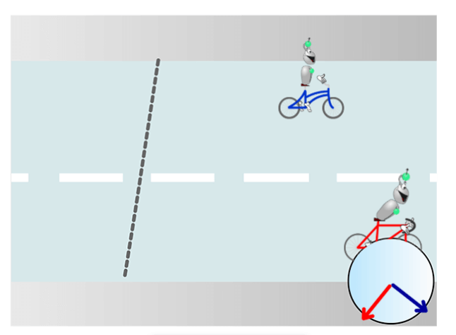
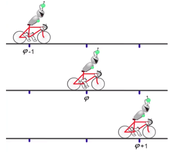
The cyclists can be differentiated according to their position after applying a gradient of difficulty. Let us take three riders pedaling side by side at the same speed: they are in phase.
We now apply a gradient of difficulty. The first will advance more slowly than the second who in turn advances more slowly than the third, resulting in distances between them. If we stop the gradient of difficulty, they will again advance at the same speed but the distance between them will be conserved.
The Frequency Gradient
The frequency gradient allows differentiating the different columns according to the rotation speed of the protons that compose it. We will now apply a third magnetic field gradient perpendicular to the first two. Protons will now rotate at different frequencies, depending on which column they are in. This is why this gradient is called a frequency gradient.
We apply this gradient at the moment of signal recovery which is why this gradient is also called the reading gradient or the readout gradient. When receiving the signal, the system is able to decompose it into several elementary signals. It is then possible to find from which column the signal originates.
The Frequency Gradient: Metaphor
When applying the gradient, the cyclists can be differentiated according to their position by their pedaling speed. But this time we are not interested in the position separating the riders but in the speed at which they are pedaling. We thus know which cyclist we are watching as a function of his pedaling speed.
Gradients Combination
What we have to remember is that when the frequency (reading) gradient is applied, the phase gradient has already been applied. The phase gradient will mark each line and the frequency gradient will mark each column.
Gradients Combination: Metaphor
Using our cyclists, the first gradient (phase gradient) separates them according to the line they are on. The second gradient (frequency gradient) allows us to identify the column the riders are in as a function of their pedaling frequency. Each rider can be distinguished by a unique distance/pedaling frequency pair.
In the first section, we will review TE and TR. It is the TE and TR parameters we use in MRI to control the appearance or contrast of the image. Recall, TE means Time to Echo and TR means Time to Repetition. We will also learn how TE and TR affect T1 and T2 contrasts, as we discuss what T1, T2, and Proton density weighting are.
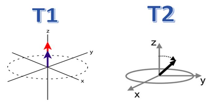
Let’s review what we have learned about T1 and T2 spins. We have learned that two things occur when the radiofrequency is applied to disturb the protons which are aligned with the magnetic field, and they occur at the same time. They are:
- T1 relaxation, or the regrowth of the magnetization back to the longitudinal direction
- T2 relaxation, or the shrinking or decay of magnetization in the transverse plane
T1 relaxation is sometimes called spin-lattice relaxation, and T2 relaxation is referred to as Spin-spin relaxation.
It is natural for the dipole of the hydrogen proton to align with the magnetic field of the magnet. In a closed bore magnet that magnetization runs head to foot, or horizontal to the plane of the table. On an open bore magnet, that magnetization runs vertically to the plane of the table. This is only important in understanding that the protons will align in a different plane on both types of scanners. The same things occur during an MRI scan, regardless of magnet types.
We will discuss in this module, ways to use the parameters of TE and TR to record the resonance of these relaxations in order to show different properties of tissue. Let’s review TE and TR first.
We know that during an MRI scan, once the RF pulse is applied, there is a period until we collect the echo. This is our TE, Time to Echo or Echo Time. We also know that during an MRI scan, we do not only apply the RF energy one time, we apply it multiple times in order to create an image. This time from one pattern of pulses and echo, to the start of another pattern of pulses and echo, is called the TR, Time to Repetition or repetition time.
TE and TR are the primary parameters that will control the contrast weighting or tissue weighting on the resulting image. There are very specific TE and TR settings depending on how the image is to be weighted. During an MRI scan, we will obtain both T1 and T2 weighted images. Another weighting we will introduce here is PD or Proton Density weighted. We will discuss this more in a bit.
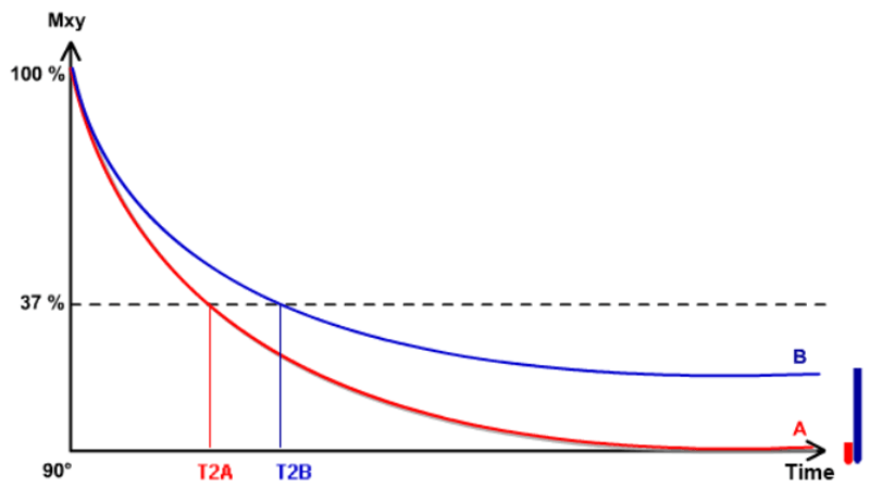
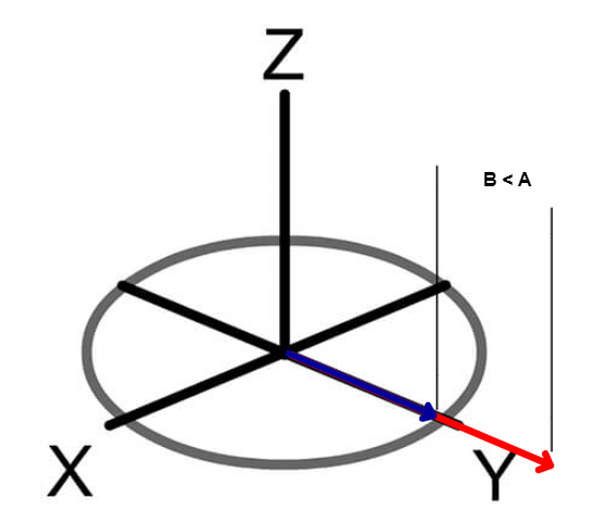
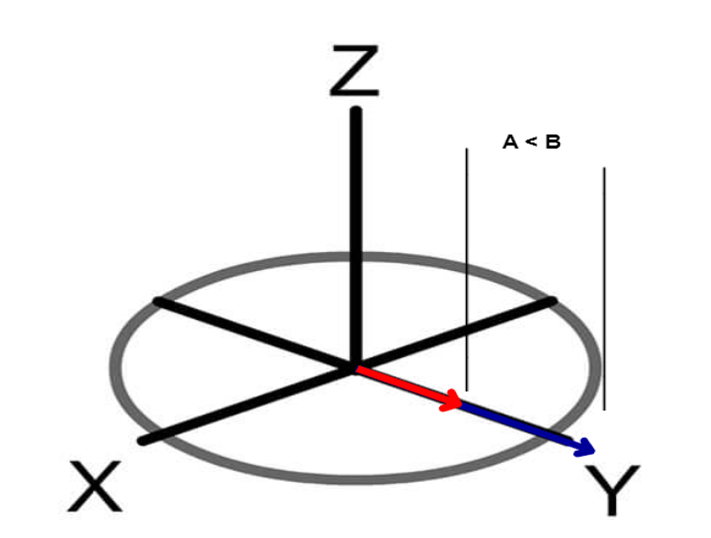
T2 Effect: Adjusting the TE
We have already seen that each tissue had its own T2 value. Here we have 2 curves that correspond to the T2 decay of tissues A and B. We are in the transverse plane which is the plane receiving the signal. As we have already explained in the introduction of the basic sequence, the signal is collected after time TE.
If we adjust the TE such as the signal is received early, we will have a good signal. However, we cannot differentiate much between the 2 tissues: their signals are very similar. Therefore, It is said the T2 effect is weak. If we adjust the TE such as the signal is received later, we will have a little less signal. However, we are able to differentiate between the 2 tissues: their signals are significantly different. It is said that the TE will affect the T2. As we have already seen, the TE adjustment affects the T2 effect. The higher the TE, the bigger the difference between the two signals of the tissues. In other words, the T2 effect is high.
T1 Effect: Adjusting the TE
We have already seen that each tissue has its own T1 value. The differences are based on the longitudinal axis. We have also seen that the signal is collected in the transverse plane only. Therefore, there should be a 90° tilt to shift the magnetization vector from the longitudinal axis to the transverse plane. This shift occurs after TR.
We should assume that the intensity of the longitudinal component before the 90° tilt determines the intensity of the transverse component after the 90° tilt.
If the TR is set so that this tilt is delayed, a lot of signals are collected because the transverse components are high. Thus, it is hard to differentiate between the 2 tissues: their signals will be very similar. It is said that the T1 effect is weak. If the TR is set so that this tilt occurs earlier, much less signal is collected because the transverse components are low. Thus, it is easy to differentiate between the 2 tissues: their signals are unique to each other. It is said that the T1 effect is high.
Therefore, the TR affects the T1 effect:
- Short TR: we increase the T1 effect
- Long TR: we decrease the T1 effect
The TR adjustment affects the T1 effect. The lower the TR, the bigger the difference between the signals of the tissues. In other words, the T1 effect is high.
The Couple TR / TE
Each tissue had its own T1 value and its own T2 value. The purpose of the MRI is to differentiate tissues:
- If the tissues are differentiated based on their T1 value, the sequence is known as T1-weighted
- If the tissues are differentiated based on their T2 value, the sequence is known as T2-weighted
The TE/TR combination gives the weight of the overall image.
Short TE and short TR:
- The short TE will result in little T2 weight
- The short TR will result in high T1 weight
Therefore, the overall weight of the image is T1.
Long TE and long TR:
- The long TE will result in high T2 weight
- The long TR will result in low T1 weight
Therefore, the overall weight of this image is T2.
Short TE and long TR:
- The short TE will weigh low in T2 contrast
- The long TR will result in low T1 weight
The difference between these tissues will only be based on the number of protons. The more proton density a tissue has, the more signal it will give. In fact, the effect of the proton density is always present (there will always be more signal in water than in air) but the T1 and T2 effects are both reduced, and only one remains. It is that of a flawed weight.
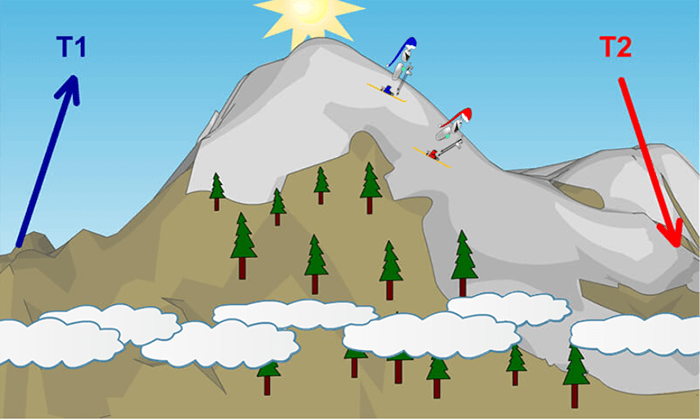
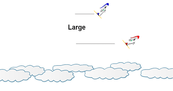
We consider that the rise of the mountain corresponds to T1 relaxation time and the descent of the mountain corresponds to T2 relaxation time. We have 2 climbers: one is fast and one is slower. If we give each of them a significant period of time, let’s say 3 months, both have had the time to reach the peak and it’s impossible to know which one was faster than the other.
If we give them a shorter period of time, maybe half a day, we will see who of them is the better climber, because he will be well ahead of the other. We consider two skiers: one is fast and one is slower. If we launch the start and take a picture instantaneously, it will be hard to determine which skier is better because they will not be far apart. If we take a picture a little later, maybe 15 minutes, both skiers will be farther apart and it will be much easier to highlight the difference between their levels.
In other words, this metaphor is very good in order to highlight the differences in terms of time scale: the T2 is much faster than T1.
Obtaining a T1 Weight
The signal is only collected in the transverse plane. Many TR and TE are required in order to obtain a sequence. Keep in mind, that what we have in a longitudinal plane before the tilt, corresponds to what we obtain in a transverse plane after the tilt.
That is why we will represent a period of time called T1 and another consecutive period of time, T2 on a different scale to allow for the interpretation. A T1 weight is obtained by using both a short TR that increases the T1 and a short TE that decreases the T2 effect. The differentiation of tissues here is mainly due to the T1 effect.
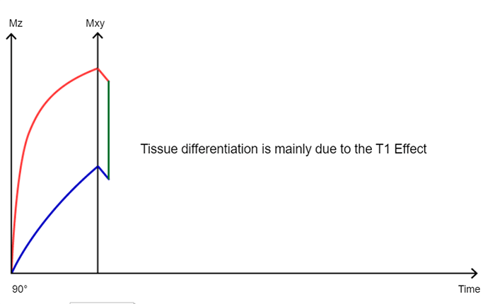
The signal is only collected in the transverse plane. In our metaphor, that is when the skiers are going downhill. This means that the picture is only taken when the skiers are skiing. However, it is impossible to highlight their separate levels as climbers.
In fact, if we give a short period of time to climb the mountain, both climbers will stop in two different areas. Then they will start descending from where they are. If we give them an equally short amount of time to descend the mountain, they will maintain this difference in the distance which will be based on their different levels as climbers: This describes T1 weight.
Obtaining a T2 Weight
As mentioned T1 and T2 happen at the same time. When it comes to obtaining a T2 weight, we keep in mind that what we have in a longitudinal plane before the tilt corresponds to what we obtain in a transverse plane after the tilt. Again, Many TR and TE are required in order to obtain a sequence.
A T2 weight is obtained by using both a Long TE that increases the T2 and a long TR that decreases the T1 effect. The differentiation of tissues here is mainly due to the T2 effect.
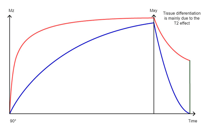
The signal is only collected in the transverse plane. This means that the picture is only taken when the skiers are skiing.
If we give a long period of time to climb the mountain, both climbers will stop higher on the mountain. Then they will start descending from where they are. If we give them an equally long amount of time to descend the mountain, the distance between them will increase and this difference in distance will be based on their different levels as skiers creating T2 weight.
Proton Density Weight
Proton Density is another weighting of tissue during an MRI scan. This uses a combination of a short TE usually less than 25ms and a long TR, usually greater than 2000ms. The short TE gives very little T2 contrast and yields a high Signal to noise ratio. This is because there is little time for the transverse magnetization to shrink. The use of the long TR gives us very little T1 contrast and high signal to noise ratio because after a long TR there is an abundance of longitudinal magnetization. As a result, neither T1 nor T2 contrast is demonstrated.
The contrast of the proton density image is dependent on the density of the protons in the area being scanned. Proton Density sequences, also known as PD, are very helpful in imaging joint spaces and the spine. As a side note, there is no clinical value or descriptive weighting for a combination of a long TE and a short TR. The resulting images would be of very low in signal and be of little use diagnostically.
T1 Relaxation Times
Recall that T1 Relaxation is The rate of regrowth of the magnetization back to the longitudinal direction. The tissues shown here are common tissues imaged in an MRI. It is important to have an understanding of the appearance of different types of tissue on T1 weighted images, as it will help to identify anatomy and pathology.
Note that Fat, has a very fast T1 relaxation time. Fast T1 relaxation has a hyperdense or bright appearance on a T1 weighted image, whereas a slow T1 relaxation will have a hypodense appearance. Therefore, on a T1 weighted image, fat would appear very bright and CSF would appear dark. All of these times are given in milliseconds.
| T1 Relaxation Times | |
| Tissue | T1 (MS) |
| Fat | 180 |
| Liver | 270 |
| White Matter | 390 |
| Gray Matter | 520 |
| Muscle | 600 |
| Blood | 800 |
| CSF | 2000 |
We have to keep in mind that the intensity of the transverse magnetization after the new 90° tilt directly related to the intensity of the longitudinal magnetization before it. Therefore, if we obtain a 90° pulse after reading a signal, the red tissue will give off more signals. The tissues with a fast or short T1 will have a hyper signal on T1 weighted images. This means they will appear brighter.
T2 Relaxation Times
T2 Relaxation, which again occurs at the same time as T1 relaxation, is The rate of shrinking of the magnetization in the transverse plane. Here we have common T2 relaxation time of tissue on MRI images. As with T1 relaxation, all tissues have their own T2 relaxation time.
Note that now, the muscle has the shortest time (T2 time that is) but CSF still has the longest. Note also, how the T2 times are much shorter. Recall from Module 3, that T2 happens much faster than T1. With T2 weighted images, a short T2 will have hyposignal Which means it will appear darker and a longer T2 will have a hyper signal which means it will appear brighter. Water will always be VERY BRIGHT on a T2 weighted image.
| T2 | |
| Tissue | T2 (MS) |
| Muscle | 40 |
| Liver | 50 |
| Fat | 90 |
| White Matter | 90 |
| Gray Matter | 100 |
| Blood | 180 |
| CSF | 300 |
We have already seen that the signal is directly related to the transverse component. Thus, if we obtain a new signal collection, tissue A will give less signal than tissue B.Tissues with a fast T2 will be in hyposignal or dark.
Contrast: The Mountain Metaphor
A good mnemonic method is to use the metaphor of the mountain. We consider that the rise of the mountain corresponds to T1 relaxation time and the descent of the mountain corresponds to T2 relaxation time.
We only consider that the closer the person is to the sun, the brighter they are. They are therefore in a hyper signal. Therefore:
- The faster climber will approach the sun more quickly in hyper signal relative to the slower climber. In other words, the tissue with the faster T1 has a hyper signal T1
- The slower skier that stays longer closer to the sun will be in hyper signal relative to the faster skier. In other words, the tissue with the slower T2 is in hyper signal T2
Examples of Weights
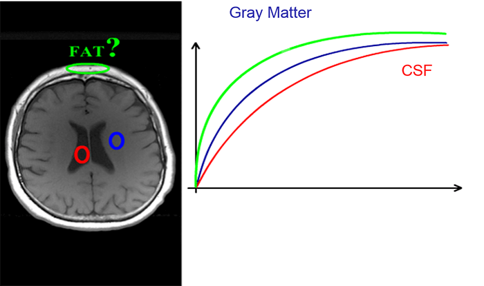
Now let’s look at how these concepts appear on an MRI image. The first example consists of an axial slice of a T1-weighted skull. The water signal or the CSF, is hypo-intense relative to that of the gray matter. Water has a longer T1 time than that of the gray matter so it appears darker.
The fat signal is hyperintense. Because it has a shorter T1 time it will show up much brighter than gray matter and water. If we display the T1 relaxation curve, we show that T1 of fat is very fast. The fat is represented by the green line, the gray matter by the blue line and the CSF by the red line.
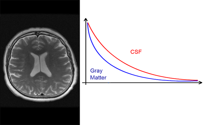
The next example consists of the same slice weighted in T2. Note that the CSF in this image is very bright. This is due to the longer T2 relaxation time of CSF. Note that the fat around the skull still appears bright on the T2 weighted image. This hypersignal of fat is not due to a long T2 time, but to another phenomenon that we will detail later.
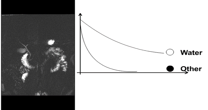
The last example consists of an abdominal image in an oblique coronal which is heavily weighted in T2. The TE is very high about 1000 ms for 1.5 T scanner. All the tissues are diffused except that of water which has a much slower T2: it is the only material to give the signal. This type of sequence is a very specific sequence that is used for studies of biliary and urinary tracts. They are used in 2D as well as in 3D.
Impact of the TR
The higher the TR, the more time tissues have to obtain their T1 relaxation time and allow the collection of the signal. On the other hand, if the TR is very short, the tissues do not have time to store the signal and will not give enough signal after the 90° tilt.
This is what we look for in certain types of sequences such as the time of flight, where the TR is very short in order to saturate the stationary tissues. These are two very important things to remember about the impact of TE and TR on the signal.
As we know, a large signal is needed to create good images. The signal has to be recorded so that it is more intense than the noise in the background. We call this signal to noise ratio. Signal must be high and noise must be low. As mentioned, if we wait too long to collect the echo, after the 90-degree pulse, the signal will weaken or decrease over time.
Thus, the more we delay the collection of the echo, the weaker it will be because of large discrepancies. Therefore we can say: the higher the TE, the weaker the signal.
Impact of TR and TE
Once again, we consider the mountain metaphor. If the TR is very weak, the climbers do not have time to pass under the clouds and thus, they will not be affected by the sunlight: they will not give the signal, they are basically blocked. If the TE is too long, the skiers have descended too much and passed the clouds, therefore they are not affected by the sunlight: they will not give signal because they are blocked.
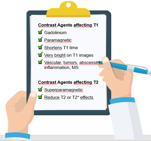
Contrast agents affect the T1 and T2 relaxation times of tissue, thus contributing to the T1 or T2 weighting on the image.
Most contrast agents affect the T1 relaxation time. These are usually gadolinium-based and are paramagnetic and will shorten the T1 relaxation time. For this reason, they will appear bright or appear to have a hyper signal on the MRI. Having this ability allows us to see tumors, inflammation, lesions, and inflammation which may be hiding behind fluid. Recall fluid will be dark on the T1 weighted image.
Some contrast are used to reduce T2 or T2* effects on an image. These contrasts are superparamagnetic. These are less common but are used. An example would be a contrast that is used for live imaging.
- The resonance is the transfer of energy between 2 systems that oscillate at the same frequency
- The LARMOR formula says w0 = gB0 (It defines the rotation speed according to the intensity of the magnetic field)
- Regrowth of the magnetization Mz is also known as T1 relaxation. The decrease in magnetization Mxy is also called T2 relaxation
- The Spin Echo sequence is characterized by the 180° pulse at TE/2. It allows it to overcome local magnetic fields inhomogeneities and raise the signal on the curve to decrease T2 true and not T2*
- The vector M will be broken into two parts influenced by distinct phenomena:
- Mz linked to excess protons in the direction of B0
- Mxy linked to the phasing of protons
- A gradient is a variation of physical size in the space
- In MRI are gradients of magnetic fields, they are linear and symmetrical
- The LARMOR’s formula said that the speed of rotation of protons is proportional to the value of the magnetic field, so a gradient of the magnetic field creates a gradient of proton’s rotation speed
- 3 gradients applied successively will allow us to locate the signal in space, they will be named:
- Slice Selection Gradient
- Phase Encoding Gradient
- Frequency Encoding Gradient (or reading gradient)
- Both the TE and TR will define the weight of an image. A T2 weighted image will have good T2 contrast, a T1 weighted image will have good T1 contrast and an image that is not either T1 or T2 weighted will have contrast depending on the density of the protons being imaged
- Also, remember that it is the TE that controls T2 relaxation and thus the T2 contrast of an image. And it is the TR that controls T1 relaxation thus controlling the T1 contrast of an image
- Contrast agents used in MRI can help to enhance the weighting of the tissue. While contrasts can be used to control T2 or T2*, most contrast agents change the T1 weighting
Post-Test & CE Certificate:
Add to CartPrice: $7.00
| ✔ | Approved by the ASRT (American Society of Radiologic Technologists) for 1.75 Category A CE Credits |
| ✔ | License duration: 6 months from purchase date |
| ✔ | Meets the CE requirements of the following states: California, Texas, Florida, Kentucky, Massachusetts, and New Mexico |
| ✔ | Accepted by the American Registry of Magnetic Resonance Imaging Technologists (ARMRIT) |
| ✔ | Meets the ARRT® CE reporting requirements |
As per the ARRT regulations, you have up to 3 attempts to pass the Post-Test with a minimum score of 75%.
Upon the successful completion of the Post-Test (score 75% or more), you will need to fill up a 1 min survey and then you will be able to issue your CE Certificate immediately.
Refund Policy: Non-Refundable
