MRI Basic Sequences
Objectives:
- Describe and identify a spin-echo from a graphic display of echoes
- List characteristics and uses of a spin echo
- List the advantages of spin echo
- Define fast spin-echo
- List effects fast spin-echo has on SAR and SNR
- Define echo train length
- Explain fat suppression and give examples and benefits of fat suppression
- Compare and contrast fat suppression and pre-saturation pulses
- List uses of gradient echo pulse sequences along with advantages and disadvantages
Description:
MRI technology is very complex, many articles and books have been written about it, therefore, it is practically impossible to discuss everything in one course. This article focuses on basic MRI sequences. The first part will address the spin echo sequence. Then inversion recovery, gradient echo and time of flight sequences will be reviewed. This article is accredited by the ASRT for 1.5 Category A CE Credits.
MRI would be simple if it were just as simple as TE and TR. We would apply a pulse we would wait a period of time, we would collect the echo and then we would repeat – measuring T1 and T2 relaxation the same way on every patient for every examination. But if this were the case, we would not get much information about the anatomy and any pathology that might be present.
Therefore, it is important to use the parameters available in MRI to manipulate the collection of data to show things differently. We call these scans sequences. There are many pulse sequences in MRI. Some of them are proprietary to MRI vendors. All pulse sequences have an acronym. Some are very interesting acronyms that spell out words. For example, General Electric has FIESTA, Toshiba has PASTA, Siemens has HASTE.
A spin echo is simply and SE; a Fast spin-echo is an FSE (although some vendors call it a turbo spin echo or TSE). An inversion recovery (we will learn more about this later) is an IR – and found in vendor sequences called FLAIR, SPAIR, STIR, SPIR, etc. Gradient Echo’s are my favorite. Only GE called a gradient echo a GE, All other vendors call them FE or Field Echo or are given the initials GRE because none of the other vendors were GE’s initials on their scanners. This is a fact!
The naming of pulse sequences can be sort of fun.
Spin Echo
The first pulse sequence we will learn is the simple spin echo or SE. A spin-echo can only create ONE acquisition at a time. Any more than that, it would be an FSE (fast spin-echo) or TSE (turbo spin echo). For this reason, spin echo’s take the most time. Spin Echo’s are the “original” pulse sequence.
A fact to remember is that T1 weighted sequences are BEST done as a Spin Echo. If an FSE is used, acquisitions or NEX should not exceed 3. We will talk more about this later. Spin Echo’s are also great for brain imaging, at least for the T1 weighted sequence.
Chronogram
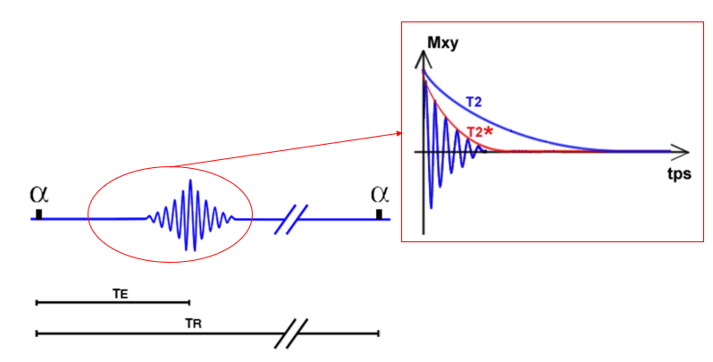
The spin-echo begins with the 90-degree pulse. The special features of this sequence are the 180° flip or refocusing pulse, occurring at half TE or TE/2. It enables us to obtain a signal that decreases according to T2 decay and not T2* decay. It overcomes dephasing due to local magnetic field inhomogeneities but not dephasing resulting from T2 against which the 180° flip is ineffective. The signal rises along the T2 decay curve after which it again decreases.
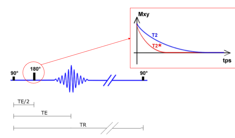
The 180° pulse
The 180° pulse overcomes the local magnetic field inhomogeneities. At the end of the 90 ° pulse, the protons are in phase. After a while, the spins had the time to undergo the phase shift. If we apply a 180° pulse. Protons continue to rotate in the same direction. If we wait again at the same time, the protons are again in phase. It is at this moment that it is then chosen to acquire the signal.
In practice, we choose the acquisition time of the signal and the system automatically sets the pulse of 180° at half of the TE or Time to Echo.
T2 Decay
Due to the 180° pulse, the signal goes up to the T2 curve then decreases again as the decrease T2*. The flip angle 180° allows us to free ourselves from the phase shifts induced by local magnetic field inhomogeneities but not the phase shift of the T2 decay. Therefore it can be traced back to the T2 decay curve but not the starting level.
Please note that an FID or Free induction decay is otherwise known as T2* decay at the end of the 90° pulse followed by a rephasing to the curve T2 followed again by a decrease T2*.
Examples
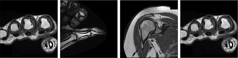
Here some examples of images made with the spin-echo sequence on various anatomical structures. As we have already discussed, this sequence is generally reserved for T1 weighting due to its acquisition time.
- Image 1 – here we have an axial T1 SE of the brain. Recall from earlier modules, the CSF is dark because of the long T1 relaxation time, and the fat around the skull is bright because it has a short T1 time
- Image 2 – The second image is a T1 SE of the thumb in the sagittal plane. Note the dark appearance of the tendon. Again, we know that means it has a long T1 time
- Image 3 – This image is a T1 SE of the shoulder in the coronal plane. We can easily differentiate between the fat and the muscle because of the different T1 relaxation times. This is what we refer to as tissue contrast
- Image 4 – this last image we have a T1 SE Coronal sequence of the hand
T1 weighted sequences are most often used for anatomical structures and anatomy. We do not get much information about a pathology from a T1 sequence.
The next pulse sequence we will review is FSE or TSE. FSE stands for Fast Spin Echo and TSE is a turbo spin echo. The purpose of an FSE or TSE is to be able to collect multiple echoes from a single 90-degree pulse followed by multiple 180 refocusing pulses and an echo that is collected after each refocusing pulse. Fast spin echoes are popular because they are faster, thus the name.
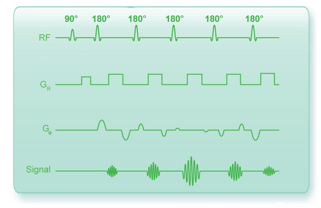
Chronogram
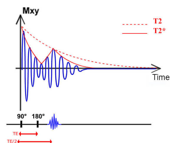
Here we have a chronological graph to describe fast spin-echo. Notice that there is one 90 degrees pulse followed by multiple 180-degree pulses, as we mentioned on the previous slide. Also notice, that there is an echo collected after each of the 180-degree pulses. The time from the first 90-degree pulse until the next 90-degree pulse is called the TR, or time to repetition. Therefore, as we see here, there can be many 180 degree pulses in one TR when using an FSE sequence. Also, note that an echo is collected after each 180-degree pulse. Therefore, we are able to collect multiple echoes in a given TR. What this means is, there can be many TE’s in a given TR depending on the type of sequence.
Important Parameters
TE is the effective TE set. It’s the echo that will fill the center of the K space. During an FSE, there are multiple 180-degree refocusing pulses. We refer to the number of 180-degree pulses as Echo Train Length. Some vendors call this echo train length, or ETL, while others call it NEX or NAQ for number of acquisitions. The longer the ETL, the shorter than the total scan time, however, the signal starts to drop with a longer ETL.
As for any spin-echo sequence, the important parameters that will condition the contrast and the weighting of the sequence are the TR and TE. However, the TE here is called the effective TE in a fast spin-echo. It is the TE which will encode the center lines of Fourier space. Indeed, the echoes will participate in the creation of the image. These are the echoes that fill the center lines which will give the information of contrast.
In a fast Spin Echo sequence, the effective TE will determine the effect of the T2 sequence:
- A short effective TE will limit the effect T2
- A long effective TE will bring much effect on T2 sequence
The TR will determine the effect of the T1 sequence:
- A short TR will bring much effect to the sequence T1
- A long TR will limit the effect T1
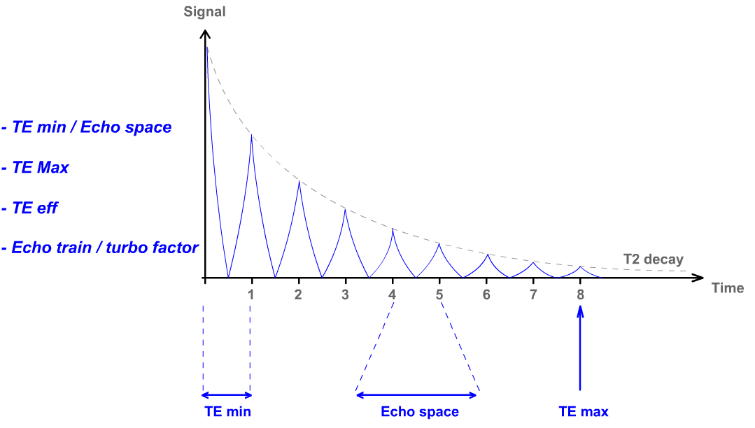
It is, however, important to consider the inter-echo space. This parameter determines the difference in the weight of each echo. Besides, this parameter will play on the last echo time (TE max). The time of this echo will determine the number of cuts allowed for a single acquisition. Another important parameter is the length of the echo train and turbo factor. It will determine the number of lines of space K which will be filled at each TR. It will also impact the T2-weighted image, the blur, and SNR.
Examples
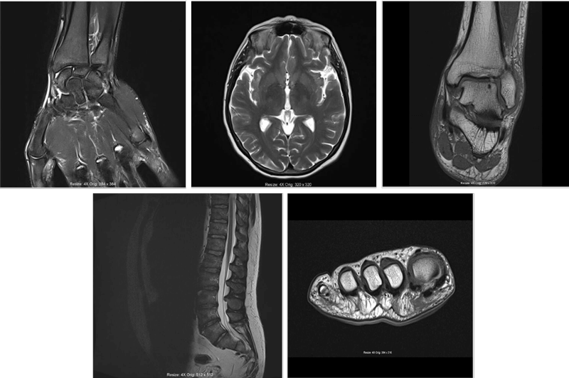
See some examples of images of various anatomy, this time made with the fast spin-echo sequence:
- Image 1 – The top image is a coronal T2 FSE of the hand, recall on T2 weighted images, fluid will be bright or hyperdense
- Image 2 – Here we have a brain image. The CSF is now bright on the T2 if you recall on a T1, the fluid is dark. This is how we differentiate between a T1 and a T2 image
- Image 3 – Here is a T2 FSE coronal ankle image
- Image 4 – Here is a T2 weighted FSE sagittal lumbar spine. Note again, like the brain, the CSF is bright. Also, note we can see these structures well without the need for any contrast in the subarachnoid space – unlike x-ray or CT scanning which requires the use of contrast injected under fluoroscopy
- Image 5 – The last image is a coronal of the foot using a T2 weighted FSE
The next sequence is the inversion recovery. We can use an inversion pulse to suppress what we don’t want to see. Typically that would be fat or fluid.
Definition and Chronogram
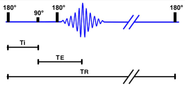
If we take the spin-echo sequence as a starting point, we have to add a 180° pulse at the very beginning in order to carry out an inversion recovery sequence. This pulse brings a new parameter into play: TI or inversion time. Ti is the time between 180° and 90° pulses. This sequence may be based on a spin-echo sequence as in our example but also a fast spin-echo or even a gradient echo sequence.
If you look at the chronology, it is almost as if we have inverted our sequence. Get it. We give a 180-degree pulse, followed by a 90-degree pulse, then another 180-degree pulse. It is important to be able to differentiate these pulse sequences from these types of graphs. This sequence is used for two main purposes:
- Better T1 differentiation among tissues
- Suppression of tissues
Better Differentiation
The 2 tissues are better differentiated according to their T1. In a spin-echo sequence, the following 90° flip, in other words, the TR, does or does not show a T1 differentiation. The 90° flip here occurs at time TI. The path taken by tissues to accomplish their T1 relaxation is twice as long which is why the difference in the rate of T1 relaxation is seen even better.
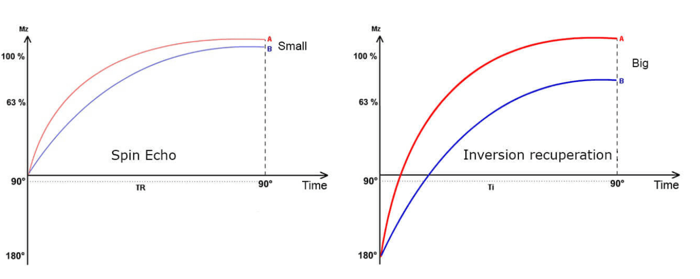
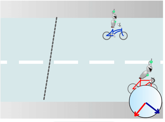
If 2 mountaineers start from the bottom of a cave, it will be easier to know who is the best. We return to our mountain where climbing is T1 relaxation.
- For the echo sequence, at each 90° flip the climbers recommence from the base of the mountain and we can see which climber is the better of the two, the one with a short T1 and thus a rapid T1 relaxation
- For the inversion recovery sequence, at each initial 180° flip, the climbers do not return to the base of the mountain but the back of a cavern. There is thus twice as much path to cover and we can more easily see which climber is the better of the two, the one with a short T1 and thus a rapid T1 relaxation
It is, however, important to consider the inter-echo space. This parameter determines the difference in the weight of each echo. Besides, this parameter will play on the last echo time (TE max). The time of this echo will determine the number of cuts allowed for a single acquisition. Another important parameter is the length of the echo train and turbo factor. It will determine the number of lines of space K which will be filled at each TR. It will also impact the T2-weighted image, the blur, and SNR.
Examples
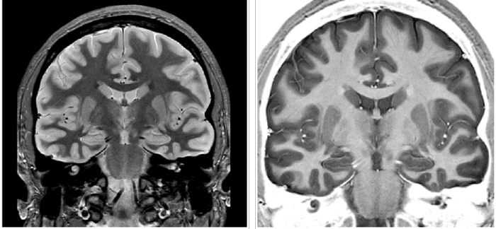
Here we have two different examples of inversion recovery. The images are of the same thing but have very distinct appearances. In the image on your left, the inversion time is adjusted so that fluid is suppressed. In this image, the gray matter of the brain appears bright and the white matter appears dark. This is because the water or fluid content has been canceled out.
In the image on your right, the inversion time is adjusted so that fat would appear to be hyperdense. It provides a white contrast background to the image and allows the brain to be visualized almost without any background. Note that the gray matter now appears dark gray where the white matter appears much lighter. That is because, though they are both Inversion Recovery sequences, they have different inversion times, canceling out different tissue types.
Tissue Suppression
The inversion recovery sequences are characterized by a 180° pulse preceding the classic sequence. The longitudinal increase occurs only at a precise moment when longitudinal magnetization is null: component Mz is also null. We must remember that what we have in longitudinal before the 90° flip we will find in transverse after it. If we set TI to 150 ms or 450 ms, we have a longitudinal component before the 90° flip, thus a transverse component after the 90° flip; the Tissue will give a signal.
If we set TI to 300 ms, the Tissue has no longitudinal component at this precise moment and will have no transverse component after the flip and will not give a signal. For each Tissue, there is thus a TI value that can be used to eliminate it. There are two principal sequences:
- STIR: cancel the fat signal with a TI = 150 ms (at 1.5T)
- FLAIR: cancel the water signal with a TI = 2000 ms (at 1.5T)
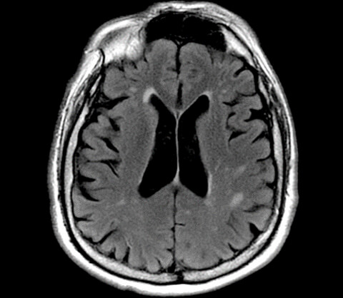
Here is an example of a FLAIR, a sequence used to suppress water or fluid. Before we talk about the sequence, we would like you not note the name. FLAIR, we know this is an inversion recovery because it has IR in the name. In the first two letters, FL tells us we are suppressing fluid.
Because there is so much fluid in and around the brain, this sequence is essential in brain imaging to look for things that may be hidden by that fluid. Note the bright lesions in the brain tissue, particularly in the parietal lobes. These are likely MS lesions or multiple sclerosis lesions. And these lesions may not have been visualized on a Spin echo or fast spin-echo. Flair is considered to be T2 weighted but notes the ventricles. On a regular T2, the ventricles would be bright because they are fluid and fluid appears bright. But we are suppressing fluid, so on this sequence, the ventricles are suppressed and appear dark. We use the appearance of the ventricles to determine that the inversion time is adequate.
There are other saturation tricks used in MRI. A fat sat can be applied as a parameter, rather than suppressed with an inversion recovery. Pre-sats can also be used and applied to the scan to suppress breathing, involuntary motion or blood flow.
Chemical Shift
The STIR sequence showed us how to cancel the fat signal. Notice again the IR for inversion recovery in the pulse sequence name. We will now examine another way to cancel the fat signal by saturating it. Let us again take a look at the water molecule and that of a fatty acid.
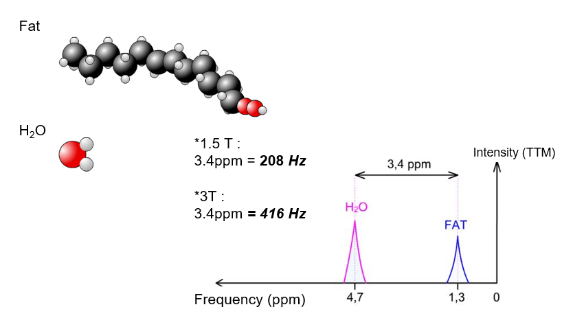
It can easily be seen that the molecular environment of hydrogen atoms is very different between the two molecules. This is why in reality hydrogen atoms do not all rotate at the same velocity when subjected to the same magnetic field strength. In other terms, the gamma of a hydrogen atom of water is not the same as the gamma of a hydrogen atom of fat.
By convention, the reference is the rotation frequency of hydrogen atoms of tetramethylsilane (TMS) and the unit is parts per million (ppm). This representation enables us to be independent of magnetic field strength. The difference in rotation velocity between protons of water and fat, in this case, is always 3.4 ppm.his value expressed in Hz is proportional to the intensity of the magnetic field. At 1.5 T this difference is 208 Hz. The higher the field intensity, the greater this difference and the easier it is to differentiate the two.
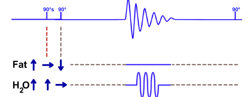
Principle of Fat Sat
We already know that in order to obtain resonance, we must have the same rotation frequency. If we apply a selective 90° pulse centered on the resonance frequency of fat: only the hydrogen atoms of fat will resonate. Fat protons are flipped 90° and water protons remain in their steady-state.
The «normal» sequence then starts. The RF pulse covers all frequencies of the section on a broader bandwidth: all protons start resonating and are flipped 90°. Fat protons are at 180° and water protons at 90° at this point. Fat protons have no transverse component and will thus not give a signal. This involves a 90° flip or fat sat for Siemens, 60° classic fat sat or 90° fat sat for GE and 100 to 110° in a SPIR for Philips, but the underlying principle is the same. There are other methods to cancel the fat signal that involve the selective excitation of water. These techniques are dealt with in a more advanced course.
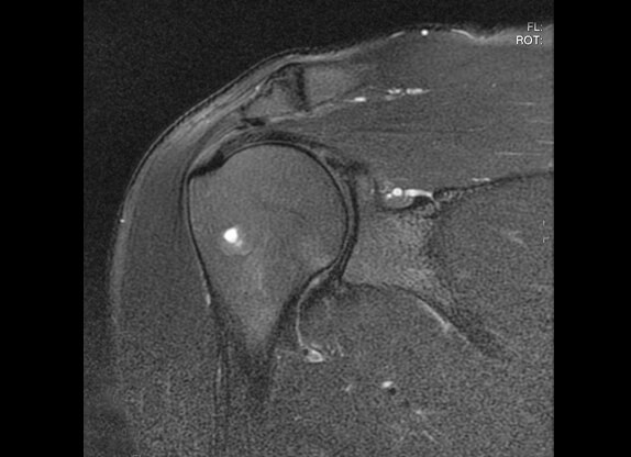
Fat Sat: Examples
This is an example of fat saturation. Fat Sats are common with extremity imaging. Removing the fat around the joint and from around and within the bone, allows us to see things that might be hidden. Additionally, it can help with diagnosis. Notice the bright signal in the humerus just below the anatomical neck. The fact we can see this on fat sat tells us that this is pathology. If it were fat within the bone it would be difficult to tell the difference between fat or pathology. We know that fat will show up bright on a T1 sequence. If we have saturated the fat, pathologies will be bright and we know they are “real”.
The fat can be removed by selective excitation based on the property that the protons of water and fat do not rotate at the same frequency.
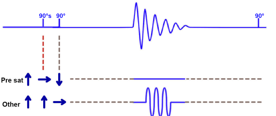
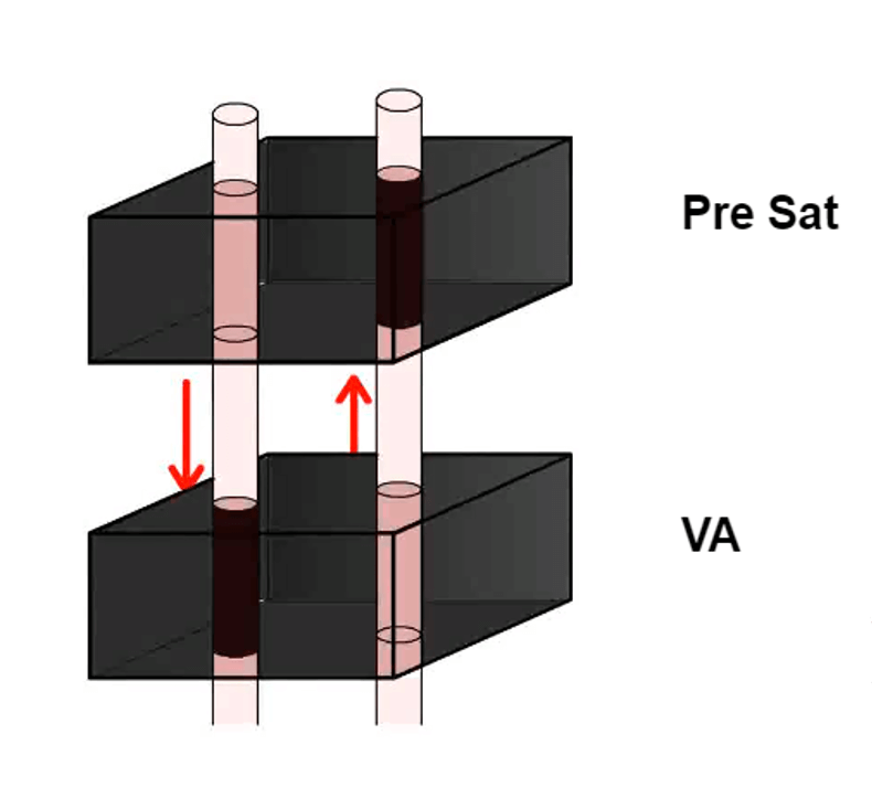
Principle of Pre Sat
In order to saturate all the tissues in a given zone, we will use a technique similar to that of fat sat. It involves the use of a selective pulse before the sequence applied (we have chosen the simplest sequence here, the spin-echo). We apply a slice selection gradient to make the protons of a precise section resonate.
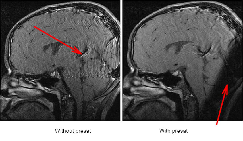
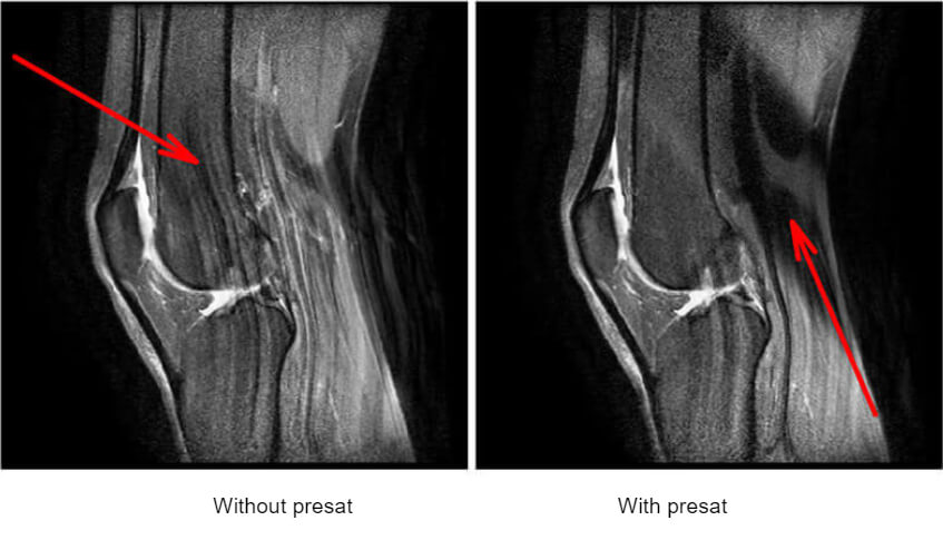
The RF wave applied covers all the rotation frequencies of the hydrogen protons of the section: all protons in the section are flipped 90° and the others are untouched. If we now apply the standard sequence. Protons inside the pre-saturation band will not have a transverse component and will thus not give a signal. These pre-saturation bands are called Sat on GE, Rest Slab on Philips or Reg. Saturation on Siemens. Example of using a saturation band to eliminate involuntary motion. The venous flow in the back of the brain is causing an artifact.
Here we have an example of using a saturation band to eliminate involuntary motion. The venous flow in the back of the brain is causing an artifact. On the second image, we see a dark band. This is a pre-saturation pulse band. It works along with the same principle of the gradients. The protons in this area will not present at the same rate as the rest of the protons in the image, thus they will not contribute signal or motion to the image.
Comparison of Fat Sat and Pre Sat
Fat sat and pre-saturation operate with similar mechanisms: they use a selective pulse just before the sequence. Fat sat sends a selective pulse to the entire volume but at a very precise frequency by adjusting the emission bandwidth. Pre-saturation sends a selective pulse overall frequencies but creates resonance at a precise location by the use of a section selection gradient.
| Fat Sat | Pre Sat |
| Selective excitement throughout the volume for a given frequency (emitive bandwidth issue) | Selective excitement for all frequencies in a given area (slice selection gradient) |
Recall another term mentioned, the Field echo because of the initials GE? Gradient echos are different than all of the other pulse sequences we have learned about because there are NO RF pulses involved in Gradient Echo sequences. The protons are disturbed by the gradients, thus the name.
Definition and Chronogram
We again take the spin-echo sequence as a starting point. There are two major differences between the gradient echo sequence and the spin-echo sequence.
- The 90° pulse is replaced by an alpha pulse with variable angles. It is a parameter that can be changed on the acquisition console: this angle will affect T1 weighting of the image
- The 180° pulse is simply eliminated: the signal will thus decrease according to T2* decay and no longer T2
The Gradient Echo sequence differs from the Spin Echo sequence, by the absence of the pulse of 180° and on the other hand by a pulse of lower or equal to 90°. TE is the time between the pulse and signal recovery. TR is still the time after which the basic pattern of the sequence is repeated With another alpha pulse – signal recovery in this case.
Gradient echoes do not use a single radiofrequency pulse. Instead, gradients are used to disturb the protons. Gradient echoes produce the LEAST amount of heat of all pulse sequences and can be popular when SAR or specific absorption ratio levels are an issue with implanted devices. A negative is that Gradient Echoes are more susceptible to the metal artifact.
Flip Angle
The larger the angle, the longer the relaxation path of tissues, and more we will be able to detect differences between relaxation velocities. Thus, the larger the flip angle, the greater the T1 effect.
If we come back to our mountain metaphor: the climbing up the mountain corresponds to T1.
- The smaller the angle is, the higher the mountaineers start their ascent
- If a = 90°, the mountaineers start from the bottom of the mountain
If we apply a 90° tipping, the mountaineers restart from the foot of the mountain and have a longer distance to cover, it is easy to differentiate the fast mountaineer, the one with the short T1) from the slow, the one with a long T1. If we apply tipping less than 90°, the mountaineers restart from a higher position having a shorter distance to reach the summit: it will be harder to differentiate between them.
Weighting
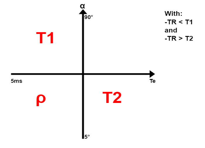
Just like we filled in a table for weightings in spin echo, we can fill in this graph with TE on the X-axis and flip angle on the Y-axis. The upper part of the graph is a zone where the T1 effect is large; the lower part is a zone where the T1 effect is small. The left part of the graph is a zone where the T2 effect is low; the right part is a zone where the T2 effect is large. TR does not participate in T1 weighting.
The fat can be removed by selective excitation based on the property that the protons of water and fat do not rotate at the same frequency.
Advantages / Disadvantages
As the table shows here, this sequence has many advantages:
- It allows generating sequence much faster than the spin-echo sequence. It, therefore, makes it possible for apnea sequences or even to create sequences in 3D
- It allows obtaining images in T2*. In other words, images sensitive to magnetic susceptibility artifacts. The aim would be to identify micro-bleeding (hemosiderin deposits) for example or cavernomas
It has the disadvantage that famous sensitivity to magnetic susceptibility artifacts. Indeed, when we do not want to highlight it, this artifact is quickly annoying. In addition, because the received signal decreases as T2*, the signal to noise ratio (SNR) of the sequence is generally lower. This is offset by the fact that the TR is shorter, the time saved can be reinvested in increasing the number of excitations.
| Advantages | Disadvantages |
| Faster than SE | – |
| Fast 3D imaging | SNR less important |
| Sequences apnea. | – |
| T2 weighting | Not true T2 imaging |
| Sensitive to low magnetic field inhomogeneities | Sensitive to low magnetic field inhomogeneities |
Derived Sequences
There are many derivatives of this gradient echo sequence. This is the case for 3D and/or rapid sequences, as well as the latest generation of sequences. The Gradient Echo sequence is the base of many sequences. The various sequences that are derived from this GRE sequence.
- TOF
- Fiesta (B-FFE, True fisp)
- SPGR, FFE T1, flash…
- Lava, VIBE, FAME…
- 3D Vascular sequences
Here are a few examples of Gradient Echoes. All are examples of 3D gradient sequences.
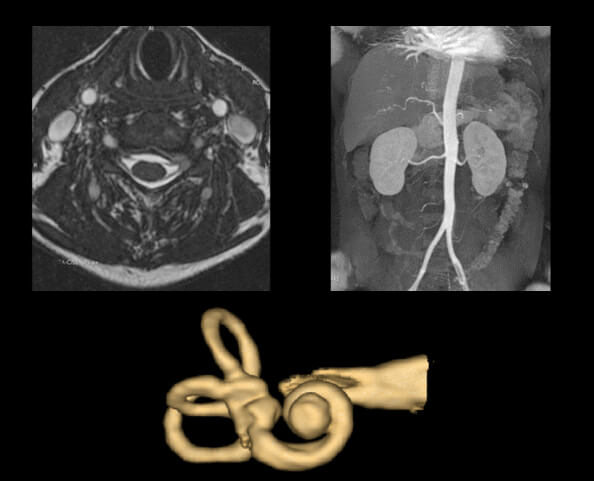
- The top left is a common Cervical spine sequence, a basic 3D Gradient T2*
- Next, we have a MIP image from a 3D TOF of the aorta. Note there is no venous flow on the image – something MRI is well known for, the ability to see the arterial flow on a 3D without venous flow
- The last image is a 3D created using a gradient echo sequence of the Ossicles in the middle ear
Last but certainly not least, the Time of Flight sequence. TOF is used to image movement or flow through a volume of tissue during an acquisition.
Definition
This is a time of flight sequence (TOF). It can be used in 2D or 3D: we will explain it for 3D but the 2D mechanism is the same. We will use very short TRs to saturate stationary tissues: tissues do not have the time to give their longitudinal increase and will thus give a weak signal during the next TR.
Blood passes through the volume: it is thus not subjected to successive pulses and will not be saturated. It will appear as a relative hyper signal with respect to stationary tissues. If we also want to saturate the signal of one of the fluxes, we will add a pre-saturation band upstream from this flux. Stationary tissues are saturated because of short TRs, and descending blood is saturated upstream by the pre-saturation band: only ascending blood will give a signal. We use this situation to analyze the Circle of Willis polygon where venous blood saturated by a pre-saturation band is extinguished.
Gradient echoes do not use a single radiofrequency pulse. Instead, gradients are used to disturb the protons. Gradient echoes produce the LEAST amount of heat of all pulse sequences and can be popular when SAR or specific absorption ratio levels are an issue with implanted devices. A negative is that Gradient Echoes are more susceptible to the metal artifact.
Adjustments TR
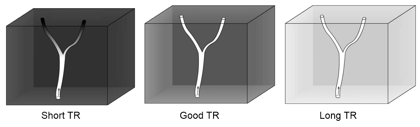
For a good TOF sequence, we must choose the shortest TR possible to saturate the stationary tissue well but we must also choose a TR long enough to allow blood to pass through the acquisition volume. Example:
- If the TR is too short, stationary tissues are saturated but the vessels are also distally because the blood that is in this place has undergone several successive pulses
- If the TR is too long, the blood has time to leave the volume and gives a good signal
On the other side, the stationary tissue signal and give too many are poorly saturated.
Examples
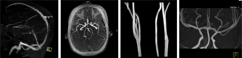
- Image 1 – Here we have a 2D TOF sequence of the venous system of the brain. Arterial flow has been suppressed by placing a pre-sat band below the brain because arterial flow comes from below
- Image 2 – This image is a 2D TOF of the arterial system of the brain. To suppress venous flow, we place the saturation band above the brain
- Image 3 – This image is a 3D TOF of the carotid arteries in the neck
- Image 4 – The last image is a coronal 3D TOF of the cerebral arteries in the coronal plane
- The sequence of fast/turbo spin echo allows us to fill several lines of K space at each TR through echo train (or turbo factor), it reduces the acquisition time
- Effective TE corresponds to the echo of the echo train which will fill the center of the K space and thus it will mainly code for the contrast of the image
- The IR sequence allows for increasing tissue differentiation in T1
- The IR sequence allows tissue suppression:
- STIR (Short Time inversion Recovery): suppression of the fat
- FLAIR (Fluid Attenuation Inversion Recovery): Suppression of water (CSF)
- The Fat Sat and the Pre Sat use a specific pulse (to avoid some signal)
- The Gradient Echo sequence doesn’t use 180° pulse, the signal is decreasing according to T2*. It uses pulses with variable flip angle less than or equal to 90°
- The flip angle will influence the T1 effect: the more it’s close to 90°, the bigger the T1 effect will be
- Regarding the TOF sequence: the TR has to be as short as possible to saturate stationary spins but long enough so that the blood bolus can completely cross the explored volume
Post-Test & CE Certificate:
Add to CartPrice: $6.00
| ✔ | Approved by the ASRT (American Society of Radiologic Technologists) for 1.5 Category A CE Credits |
| ✔ | License duration: 6 months from purchase date |
| ✔ | Meets the CE requirements of the following states: California, Texas, Florida, Kentucky, Massachusetts, and New Mexico |
| ✔ | Accepted by the American Registry of Magnetic Resonance Imaging Technologists (ARMRIT) |
| ✔ | Meets the ARRT® CE reporting requirements |
As per the ARRT regulations, you have up to 3 attempts to pass the Post-Test with a minimum score of 75%.
Upon the successful completion of the Post-Test (score 75% or more), you will need to fill up a 1 min survey and then you will be able to issue your CE Certificate immediately.
Refund Policy: Non-Refundable
