MRI Image Creation and Quality
Objectives:
- Describe the process of collecting the signal at the coil through the digitizing of the data and image creation
- Define Fourier transform
- Describe and identify the matrix, including phase and frequency of the matrix
- Define pixel
- Describe k-space and how k-space is filled
- Identify what aspects of k-space are responsible for contrast resolution and spatial resolution
- Define NEX
- Compute acquisition times
- List the primary parameters used in MRI and how they each relate to image quality
- Describe computer controls that affect image quality
- Match types of pulse sequences to their associated image contrast
- Define SNR
- Identify noise on an MRI image
- Define spatial resolution
- List parameters that affect spatial resolution
- List parameters that affect SNR
- Select appropriate trade-offs to balance image quality and SNR
Description:
In this course, we will discuss how the data is collected and transformed into an image in MRI. Image quality is important, and because an image of poor quality can hide a pathology and lead to misdiagnosis, in this article we will also get to learn and understand what makes a good quality image, and how the parameters selected can affect the image quality. Image quality is important, because an image of poor quality can hide a pathology and lead to misdiagnosis. This article is accredited by the ASRT for 1.25 Category A CE Credits.
Data collection begins at the coil. Recall that the coil acts like an antenna that captures a radio wave. In our words, the coil is capturing the resonance wave or the echo.
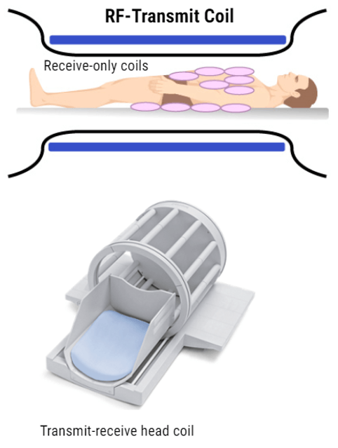
MRI Coils
We now understand that during the process of MRI, the resonance in the form of an echo wave is given off during the relaxation of T1 and T2. In order to create the image, we need to collect that echo. In MRI we use very special equipment called Coils. The coil acts like an antenna so to speak, similar to the way an antenna on a car might pick up the radio waves being transmitted from radio stations.
There are several different types of coils, some are specifically designed for specific body parts, and some are capable of being used for any type of imaging. Also, a coil can be classified as a receive-only. What this means is the coil may ONLY receive the signal but does not transmit – for these types of coils, the transmission of the RF energy comes from the inherent body coil of the magnet.
A coil can also transmit and receive. A transmit/receive coils do both functions – transmission of RF and Receiving of the echo. These types of coils are also referred to as “local transmit coils” because of their proximity to the body part. The only thing we cannot have is a transmit-only coil. Even the TR body coil can transmit RF energy and Receive a signal.
General Principle
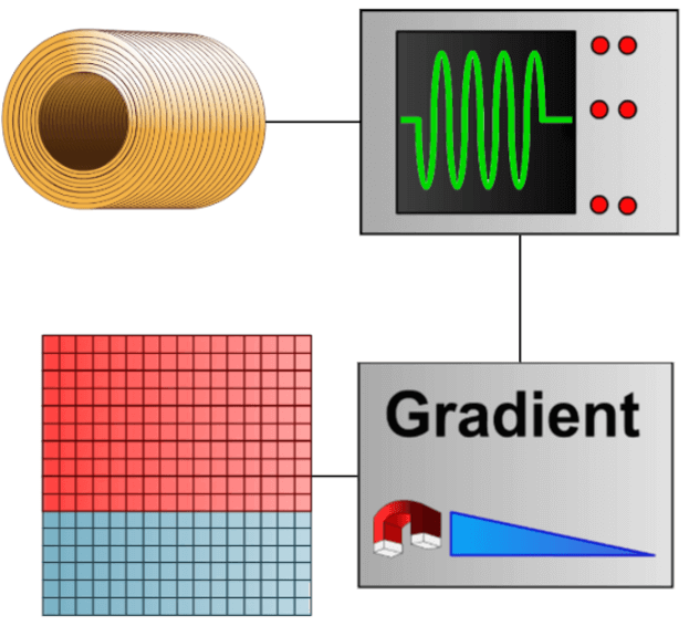
An RF wave is emitted, a signal is sensed and thanks to the use of the gradients, this signal is used to fill the mathematic space called Fourier space or K space. Once the K space is filled, we apply a mathematic formula that is a Double Fourier Transformation to obtain an image. The Fourier space is the frequential representation of the image.
The general principle of MRI can be summarized with a magnet, a radio frequency wave, a signal that is sensed, which is localized and treated through the use of gradients. This signal is used to fill a mathematical space called the Fourier space. We then get an image using a mathematical formula. These mathematical formulas are called algorithms.
K Space
The Fourier space (K space) is the place where we store and sort the recorded signal. For this Essential MRI course, the take-home message is simply that the Fourier space is where the system stores information in the form of a signal. This is like thedog that arranges objects in his doghouse. Remember Hydro? We can see him through the window of the house. And this is his dog. He is placing slippers on one side, and bones on the other side. So in a sense, he is sorting through the things he is finding in the yard.
Matrix or Battleship
The signal is arranged in the matrix like the ships in a game of battleship. The system sorts information according to their phase and frequency. Just like the game of battleship where the ocean is a grid of letters and numbers, the MRI Fourier space is a grid of phase and frequency.
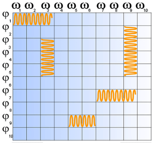
Reference Frame of Frequencies
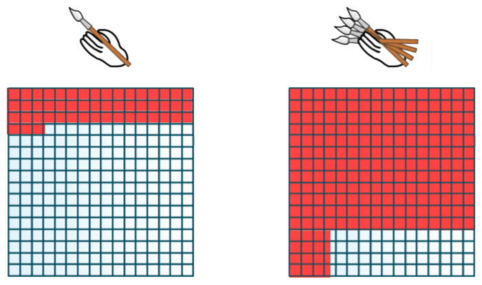
The K space is the frequential equivalent of the image which is a spatial representation. Example: We take one white square for which we decide to blacken every other box going toward the right and one out of 3 boxes going toward the bottom.
This process is repeated until We fill in the entire grid according to this rule. Consider the horizontal filling to be the phase and the vertical to be the frequency.
The space of the localization domain and frequency is referred to as “Fourier Space”. Fourier space is needed so that when the image is created from the data collected, the computer knows where each bit of information belongs. Similar to putting together a puzzle. If the pieces are not arranged in the exact order they were intended, the image will not look like the object it represents.
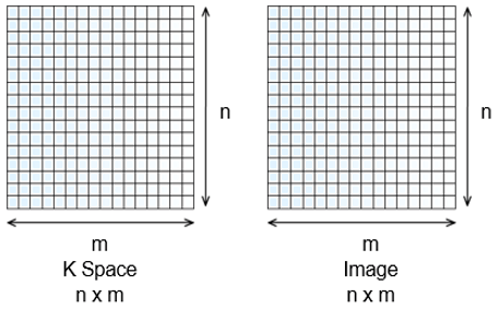
Dimensions of the K Space
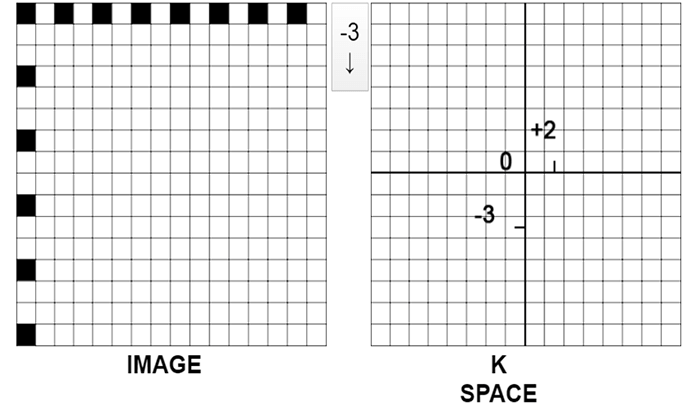
The dimensions of the Fourier space and the image are the same. This means that the size of the field and the size of the matrix we set in the scanner parameters are in fact the size of the FOV and the matrix of the Fourier space. It is the acquisition matrix. In reality, the image is reworked before restitution or reconstruction. In general, the image restored is a 5122 image. The size of the matrix represents the number of pixels or the number of tiny squares inside the large square. On a 512 matrix, there will be 512 rows of pixels and 512 columns of pixels.
Pixels of the K Space
Each pixel of the Fourier space codes for all pixels of the image. In other words, in each of the pixels of the K space, we will have information on all the pixels of the image.
![]()
Pixels of the Image
Each pixel of the image has been coded by all the pixels of the K space. In other words, each of the pixels of the image has received information from the entire K space.
![]()
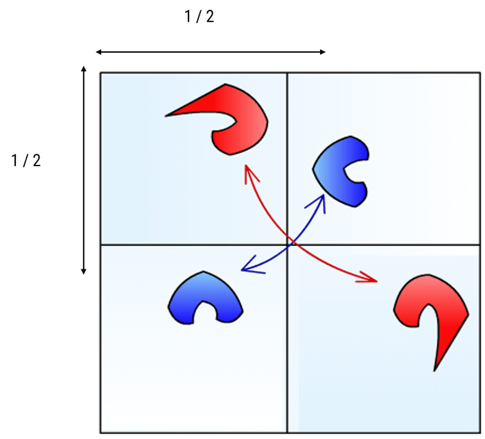
The symmetry of the K Space
The space of Fourier is divided into 4 symmetrical parts, 2 by 2.The K space is symmetrical according to a complex conjugated symmetry around the center. This property is used for rapid sequences for which we fill in only half the Fourier space and the other half is mathematically deduced. This is the case for single-shot fast spin echoes known as SSFSE or Haste sequences. Haste stands for “half acquisition spin turbo echo.
Center and Periphery of the K Space
One of the most important properties of the Fourier space is that the center contains information on contrast and the periphery contains information on spatial resolution. This notion is indispensable for understanding the notion of effective TE and for understanding how filling the Fourier space differently can be used to create specific vascular sequences.
When we want to have an acquisition coincide with precise vascular time, in other words, arterial for example, it is important to have the acquisition of central lines of the K space coincide with the passage of contrast product at this precise moment.
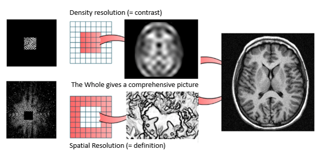
Contrast and Resolution
To summarize, the center of the K space codes for the contrast resolution. Whereas, the periphery of the K space codes for the spatial resolution.
Filling the K Space
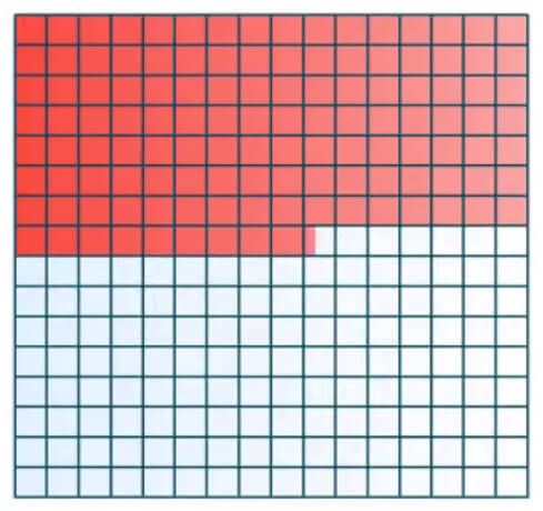
In most sequences, the Fourier space is filled in line by line: this is called linear filling. For other sequences, space is also filled in line by line but starting at the center: this is the centric mode. GE and Siemens scanners use this. Or Linear Low-High as it is called on Philips. This filling can also be done starting in the center but in a centrifugal manner or snail-shaped. This is centric elliptical mode common on GE or Siemens scanners or central as referred to on Philips.
Acquisition time is important. MRI scan sequences can be long. We can adjust parameters to minimize time. This is helpful for claustrophobic patients, or patients who are in a lot of pain.
The Acquisition Time Formula
The time of an acquisition is the time required to fill the Fourier space, multiplied by the number of times we want to fill the space. To start, we take a sequence which is filled linearly. The time needed to fill a Fourier space is the time to fill in one line multiplied by the number of lines.
In reality, the space of one TR is needed to fill one line and we have as many lines as indicated by the phase matrix. Another parameter involved is the ETL or echo train length or turbo factor as it is sometimes called. It is the number of lines of the Fourier space filled in at each TR. The number of Nex is the number of times the Fourier space will be filled. A good analogy for the number of Nex’s is a painter repainting a wall: the more coats of paint, the better the result but more time is required to fully paint the wall.
ETL (echo train) = TF (turbo factor)
The Echo Train
The echo train (=turbo factor) corresponds to the number of lines of the K space that are filled during each TR. The acquisition time is reduced accordingly.
Example: The parameter is equivalent to the number of paintbrushes used by the painter: the more brushes (the higher the number), the more the lines of the Fourier space can be filled in during one TR and so the entire Fourier space will be filled in more rapidly.
In our example, if we use 4 brushes (turbo factor or ETL = 4), our Fourier space will be filled in 4 times more rapidly. This is a concept we discussed when we learned about the fast spin-echo sequence.
We have been discussing a single slice in a single acquisition. Scanning that way can take a long time, and for a while, that was all MRI was capable of. There are ways, using parameters in the scanner, to acquire several slices in each acquisition.
Chronogram
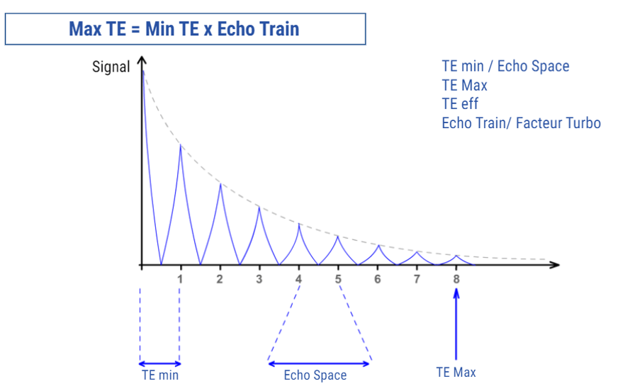
The time between the end of receiving a signal for an image, or MAX TE, and the moment of application of the 90° pulse (TR) is used to obtain a second diagram or a single echo, with the same parameters. In fact, the number of slice diagrams allowed per slice depends on the TE Max and the TR.
It is possible to change the size of the Max TE and the TR and visualize its impact on the number of slice diagrams obtained. If the TR is an easily accessible and comprehensible parameter, this may not be the case with the Max TE which does not directly respond. Besides, the parameters that impact Max TE are not the same and are based on the device. By increasing the TR or decreasing the Max TE, we can obtain more slice diagrams in a single acquisition.
The Maximum TE
The Max TE corresponds to the last echo in the echo train. In fact, its value corresponds to the time that separates the echoes, the time between echoes or TE, multiplied by the number of echoes obtained at each TR (ETL). This Max TE is not a parameter that can be accessed directly but it can be indirectly modified by modifying the echo train or by modifying the minimum TE. Based on the manufacturers, the parameters that affect the Maximum TE might not be the same. In fact, they don’t all adopt the same philosophy in terms of the automation changes.
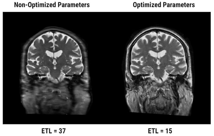
Blurring
Description:
There are a few artifacts associated with multi acquisition scanning. Here we have Blurring. This artifact is characterized by an image whose spatial resolution is poor despite the small size of voxels. All the edges are blurred. While it may have the same appearance, it is important to not confuse blurring with motion artifact or a simple poor spatial resolution.
Origins:
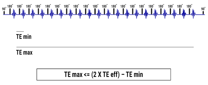
This artifact is due to a very large difference in weight between the effective TE (TE eff) which will mark the center lines of the Fourier Transform and the weight of the last echo in the echo train or Max TE, which will mark the peripheral lines of the K-space.
When the difference between the weight of the echo that fills the center and the echoes that fill the periphery is too large, this blurring artifact appears. In an optimum setting, the Max TE should not be more than double the TE eff minus the TE min.
Optimizing the Effect:
To reduce the blurring artifact, the effective TE must be in the center of the echo train. Based on the manufacturers, the parameters are more or less automated. Some systems automatically alter the values of inter-echo space so that Max TE is double the Effective TE. Some allow full control, which implies a knowledge of this problem. Some others still leave some room for maneuver or adjustment to parameters.
Next, we will develop the rationale for a system that doesn’t have any automatic mechanism in order to properly identify the different aspects of managing these parameters
Chemical Shift
Description:
The next artifact is the chemical shift. This artifact is visible at the level of a water/fat interface in order to code the frequency. One side of the liquid object in a fatty environment shows that its outline is enhanced by a hyper signal border. However, the opposite is enhanced by a hypo signal border. This can also appear for a fatty object in a liquid environment. This artifact is for coding the frequency: it is called the chemical shift.
On this image, look at the areas where the red arrows point, and you will see the effect of chemical shifts around the kidneys.
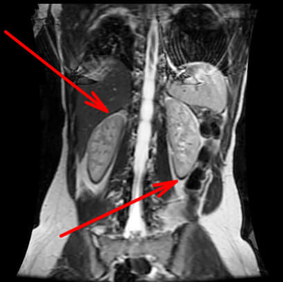
A strip of hypo and hyper signals on each side of the water / fat interface in order to code the frequency.
Origins:
We have seen that the protons that are exposed to a magnetic field rotate with a specific frequency which is Larmor frequency. In fact, the molecular environment of Hydrogen protons will slightly impact their precession frequency. This difference in rotation speed will be the source of this chemical shift artifact.
The difference in the rotation speed of the Hydrogen protons of water and fat is always 3.4 ppm. This means that for a magnetic field of 1.5 T, the difference is 208 Hz. We have seen that the signal was moved by Fourier Transformation by its frequency. Because of this difference in the rotational speed of the water protons relative to those of fat, they will be artificially shifted against each other.
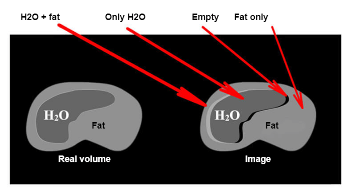
If this 208 Hz are shown in more pixels, then these signals will be located in the wrong position. Notice that around the organ, there will be a part where the signals of water and fat will add up (H2O + fat = white stripe), a part where there is no organ (H2O = normal signal the organ), and a part with no signal (nothing = black band). This is the chemical shift.
Bandwidth and Chemical Shift
The bandwidth represents the different frequencies contained in the signal. These frequencies cover all the FOV and are distributed according to the frequency matrix. Based on the manufacturer, the bandwidth can be adjusted according to the variation of both sides of the center, The number of Hz per pixel or the number of pixels covered by the chemical shift.
Receiver Bandwidth
One thing about bandwidth. The larger the bandwidth the more noise that will be allowed into the image. When the bandwidth is increased, more noise is within the bandwidth. Noise, as we will learn in module 7, it detrimental to the image quality.
When noise is increased, the signal is decreased. But, it does decrease the inter-echo space which allows more slices in an acquisition. It is important to balance all of this. Always remember. The signal should always be higher than the noise.
The Frequency Matrix
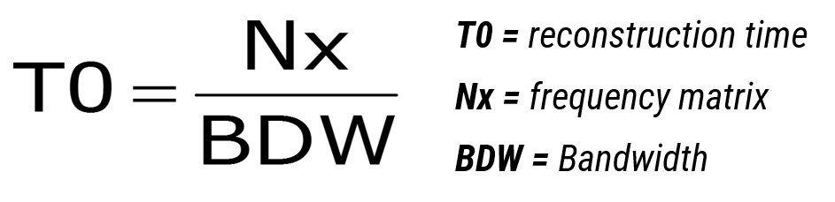
While reading the signal, a magnetic field gradient is applied. Thus, the received signal is composed of several signals, each having a particular frequency. The frequency matrix corresponds to the number of different frequencies that make up the signal. In fact the size of this matrix influences the reconstruction time. The higher the number of frequencies in a signal, the longer it will take for the system to view it.
Reconstruction Time
The inter-echo space depends on the reconstruction time. This is why the frequency matrix and the bandwidth have one impact on the inter-echo space. In fact, these parameters impact Max TE and the number of allowed slices per acquisition.
In this formula, the reconstruction time is equal to the frequency matrix divided by the matrix. As you can see both of these parameters have a direct impact on the time it takes to reconstruct an image.
Summary
It is important when making changes to parameters to have a good understanding of the effect of those changes have on things, such as time, spatial resolution, contrast and signal to noise. On this slide, you can make changes and see what the direct impact would be. For example, We can see the different parameters that should be modified in order to obtain more slices in the same acquisition.
There are several available solutions:
- Increase TR: contract T1 should be monitored, as well as the acquisition time
- Decrease the echo train or turbo factor: the acquisition time should be monitored here too
- Increase the bandwidth: the problem is the impact on the signal to noise ratio
- Decrease the frequency matrix: the decline of spatial resolution should be monitored too
Also, certain devices do not directly give access to the bandwidth that automatically adjusts to the inter-echo space so that the effective TE situates in the center of the echo train. But rather, the bandwidth is automatically defined based on the turbo factor, the effective TE, the frequency matrix, and the number of pixels of chemical shift.
The contrast in an image is the ability to resolve structure in relation to other structures in close proximity or to resolve a small difference within a structure. In x-ray contrast is controlled primarily by KVP selection, and is affected by the attenuation of the beam. In digital radiography, the detectors and bit depth of the detector elements play a role.
In MRI contrast is a little different. There is no attenuation in the MRI. In MRI many factors control signal and contrast. Contrast is first controlled by TE and TR, resulting in Proton Density, T1 or T2 weighted contrast. Image Contrast is also determined during the filling of the center of K space. By definition, contrast is the ability to differentiate differences in signal intensity of adjacent tissues.
The contrast of an MRI image depends on several factors including the parameter settings that affect weighting; such as. TE, TR, TI, flip angle as we have learned in other modules. Also, factors such as the mechanism for filling the Fourier space during reconstruction, filters used during reconstruction, and selections of window width and window level or window center used during image display. It is important to maximize the contrast between tissues in order to be able to distinguish between them visually.
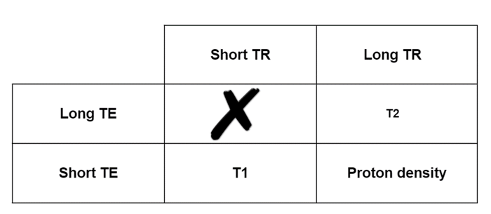
Contrast, in MRI, can be described as the ratio of the magnetization of two tissues. In the simplest terms, contrast is most often referred to by the predominate weighting. T1 weighting, T2 weighting or PD weighting. NOTE that the short TR and Long TE results in a useless image.
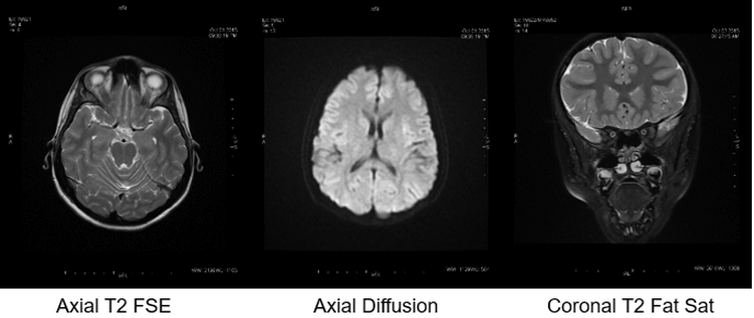
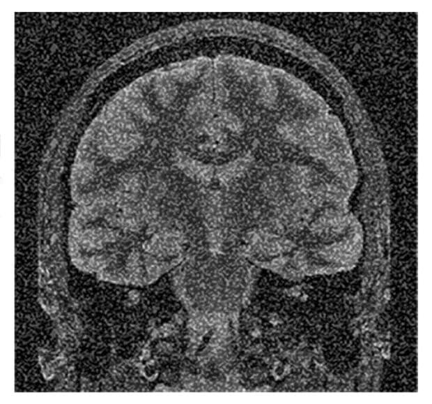
Here we are looking at a variety of different ways to show T2 weighted contrast. In the first image, we have an Axial (which tells us which plane we have acquired the data) T2(which tells us which tissue contrast we have acquired), and the acronym FSE (which tells us that it is a Fast Spin Echo). The second image is also an Axial, and it is T2 weighted, however, it is a diffusion scan which is producing an image that takes into account how well the brain tissue is diffused with blood. As you can see they look quite different and are showing us very different information.
The last image is also a T2 weighted image, however, it is a coronal and we have applied a Fat Saturation pulse to the sequence. If you look closely around the skull on the first and last images, you can see the fat surrounding the skull is NOT visible on the last image, and it is visible on the first image. Remember, T2 weighted images are heavy on T2 contrast.
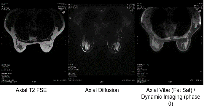
This set of images of the breasts is also T2 weighted. Again, we have a T2 FSE, and Axial Diffusion and a variation of the Axial T2 Fat Sat. If you recall in module 5, we learned that all vendors have proprietary pulse sequence names that are unique to them but describe pulse sequences used by all vendors. Here, the fat suppression is slightly more pronounced than on the previous slide of the skull.
In the first image, we see that the breasts are composed mostly of fat. Fat is relatively bright on the T2. In the Fat Suppressed sequence in the last image, the fat is now dark, because it has been suppressed. Again, all three images display T2 contrast, but in different ways.
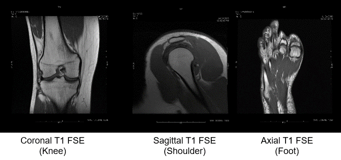
Now let’s look at some T1 weighted contrast. T1 contrast mostly shows anatomical size, shape, location. T1 (without the use of contrast agents) is usually used to display anatomy, not pathology.
Here we have a Coronal view of the knee, a sagittal view of the shoulder, and an axial view of the foot. All are Fast Spin Echo’s as we see the FSE indication. As you can also see, T1 weighted contrast has a very different appearance compared to T2 weighted contrast on an MRI image.
Signal to noise ratio, SNR or simply S/N is extremely important. Noise is detrimental to image quality. If an image is excessively noisy we say that it is starved for the signal. Most, if not all, of the parameters discussed in the previous module, affect the signal. If a parameter decreases signal, noise automatically increases.
Keep in mind, the amount of noise is consistent from sequence to sequence. It is the amount of signal that is dependent on the parameters selected by the technologist. It is desirable to obtain a large signal while minimizing the visualization of the noise. One important thing to note: SNR is optimal when it is 100%, but keep in mind, that SNR should never go below 80%, otherwise the image is too greatly compromised.
Definition
The noise is the whole of the incoherent signals which degrade the formation of the image. In MRI our goal is to have High signal and low noise in the final image. Any parameter or other factor increasing the amount of signal given off by the body OR measured by the scanner, will in turn increase signal.
We refer to this as the Signal to Noise Ratio or SNR. If the signal increases and/or noise decreases, the signal/noise ratio increases. If the signal decreases and/or noise increases, the signal/noise ratio decreases.
Significance of Low SNR
Notice the appearance of the image.
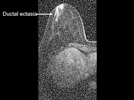
As you know previously, the metaphor of the dance club. The signal must be greater than the background noise in order to be heard. Here we have an image of the breast with a pathology called ductal ectasia. While we can see that there is an abnormality, especially the borders. This is important. If there was a small lesion present, the noise may completely obscure it.
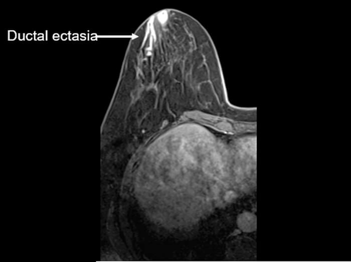
Significance of High SNR
As you can see it is much easier to see the anatomy get a full appreciation of the weighted contrast in images with good signal to noise ratio. We can also get a lot more information about the pathology and the extent of the pathology. Doesn’t this image look much better than the one on the last slide.
When Noise is Acceptable
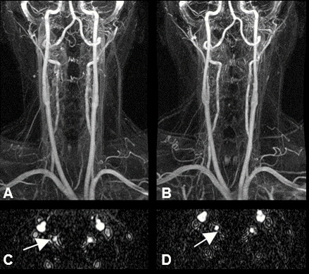
Some image sequences will inherently have more noise than signal. Most are 3D images that will require post-processing to make it look “better”. An example is the 3D collection of data during vascular imaging. The MRI contrast media will provide most of the signal, and as the image data is processed and the unusable portions of the image are cut away, the image will have an appearance of less noise.
Basically speaking, it can be said that the noise is processed away, so it does not matter that it appears in the original set of data or the raw data. Here, in C and D we see the unprocessed, raw data images, which are processed into 3D model. In this instance, the raw data that is acquired during the scan is of low signal, which is acceptable to a degree. As can be seen, the processed images above in A and B look much better.
Parameters Affecting Signal
Matrix:
Matrix affects signal in the sense that the larger the matrix, the lower the signal to noise ratio. This is because a larger matrix has smaller pixels. While smaller pixels are good for spatial resolution, they are not so good for the signal. Consider having a cracker and a slice of bread. You only have a teaspoon of jelly. Which would it cover more completely? The cracker because it is smaller. If we have to spread the signal over a larger area or cover more pixels we would lose signal, or have decreased signal. Any time signal decreases, noise increase and we express that as a lower signal to noise.
ETL:
The echo train length will affect SNR. With a longer ETL, we are collecting signals over a longer period. As time passes we know that relaxation is ending – especially T2 contrast which happens faster. Therefore, if you can imagine, the more time that passes, the lower the amount of signal coming from the proton’s resonance. The longer the ETL, the lower the signal to noise ratio.
Slice Thickness:
Decreasing slice thickness will decrease SNR. When the collected slice thickness is very thin, we have a limited amount of protons in the slice selection to contribute to the signal. Therefore thinner slices = more noise, and vice versa.
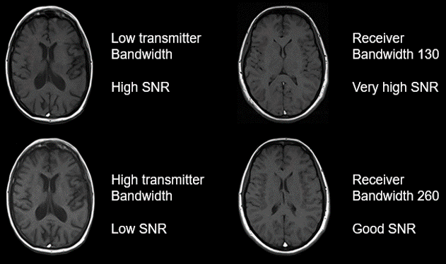
Bandwidth:
In MRI the bandwidth is the number of frequencies that are either transmitted or received in a period. The transmit bandwidth is the width of the transmitted. It is usually more narrow than the receive bandwidth to ensure the signal does not spread beyond the receive bandwidth.
Think of x-ray and beam collimation. More narrow beam collimation provides that the radiograph would have better detail, whereas a beam that is not collimated leads to scattering which appears as noise or quantum mottle on the radiography. Therefore, narrow or low transmit bandwidth results in higher SNR. The receive bandwidth is the opposite. Because the receive bandwidth represents the number of frequencies measured, a narrow receiver bandwidth will result in a higher SNR.
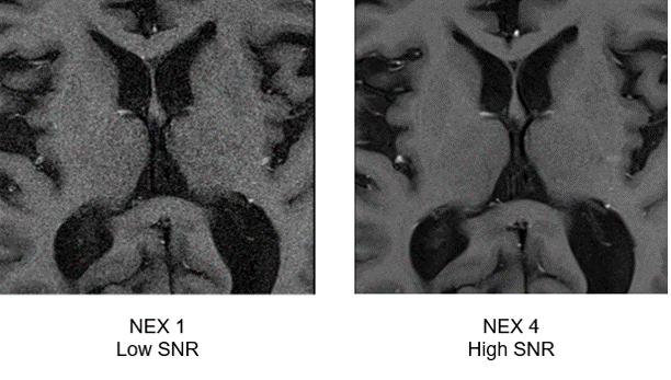
NEX:
The final two parameters affecting signal are NEX, or several acquisitions, and TE. NEX is simply the number of times the same area of protons is sampled or acquired. The more times we sample something, the better the signal. Some vendors call this “number of signal averages”. It is important to remember, however, that the higher the NEX, the longer the scan time. Compare the two images above. Note the difference in signal between the NEX of 1 and NEX 4.
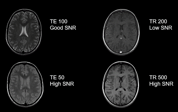
TE and TR:
Recall TE means “Time to Echo”. Also, recall that the longer we wait to collect the echo, the weaker the signal because as time passes T1 and T2 relaxation come to an end. For this reason, a short TE will give a stronger signal than a longer TE. Compare the images to the left. Note that both images have decent signal, though the image with a TE of 50 has higher SNR. However, notice the difference in T2 contrast – because TE also controls T2 contrast it is not always the parameter of choice to change to control SNR and can only be changed within a range that will not change the desired contrast of the image.
While TR does not directly affect the amount of noise in an image, it needs to be discussed here because longitudinal magnetization will allow SNR to be at its greatest appearance. A longer TR, or time before repetition, allows for more recovery thus allowing for greater longitudinal magnetization, thus optimizing Signal to Noise ratio. However, notice the difference in T1 contrast – because the TR controls T1 contrast it is not always the parameter of choice to control SNR, and only can be changed within a range that will not alter the desired contrast of the image.
Keep in Mind
When performing MRI, tradeoffs are inevitable. So it is important to keep a few things in mind when making these decisions because there is always a trade-off. Parameters that improve one aspect of image quality will have a negative effect on another. When it comes to SNR, the greater the amount of sampling or the more frequently something is sampled, the greater the SNR.
This would be a simple decision because good SNR is preferred. However, most of the parameters which give better SNR, will increase the scan time or decrease spatial resolution or BOTH. Therefore, we look at just the effect on SNR for this portion of the discussion and remember that:
- Thicker slices give a better signal to noise ratio
- Smaller matrix gives a better signal to noise ratio
- Increasing NEX will give a better signal to noise ratio
- Decreasing TE will give a better signal to noise ratio
- Increasing the bandwidth will give a better signal to noise ratio
- Decreasing the transmit bandwidth will provide a better signal to noise ratio
We mention again, this is without making any other changes to any other parameters to compensate.
As we have seen, parameters can be used to increase the signal available to create an image. And we have mentioned that some of these adjustments will have a detrimental effect on Spatial Resolution. Just what is spatial resolution then? Spatial resolution or just resolution is another very important quality factor when it comes to MR imaging. Spatial resolution is defined as the ability to visualize very small objects. MRI is famous for its spatial resolution.
In MRI, we can often see tiny nerves easily, therefore it is a very important aspect of image quality. In X-ray, we often refer to spatial resolution as detail. As you will see as we progress, that signal is compromised when we try to optimize spatial resolution, and vice versa. Spatial resolution is expressed in lp/mm when image quality is tested. A conceptual idea to remember is that anything that happens more frequently has a higher spatial resolution. We are going to look at parameters individually, and relate them back to this concept.
The Matrix
The first parameter associated with the spatial resolution is the matrix size. The matrix is the number of rows and columns of pixels. A large matrix provides the best spatial resolution. This is because with a large matrix we have more rows and columns, therefore the signal is sampled more times in a given distance of space considering each pixel will be sampling and the fact that each pixel is smaller. Smaller pixels = better spatial resolution.
This is true provided the size of the field of view (FOV) remains the same. Therefore, if the size of the FOV is constant, by increasing the size of the matrix, the pixel will be smaller. Thus the spatial resolution will be higher. Keep in mind, the opposite would be true – a lower matrix would decrease spatial resolution, again, provided the FOV stays the same. Recall if the matrix is increased there are more pixels in a given space, which means the pixels occur in higher frequency which means higher spatial resolution.
The Field of View
Likewise, if the matrix stays the same, but we change the Field of view, we can also affect spatial resolution. A smaller FOV will give a better spatial resolution. Besides, if a large FOV is used, the image would need to be magnified on the monitor – causing each pixel to be magnified, thus reducing spatial resolution.
Using a small FOV allows us to magnify the anatomy by placing the data across the monitor without changing the appearance of the pixels. Again, because FOV and matrix are related, a smaller FOV means we have smaller pixels. Smaller pixels mean each pixel must be smaller. Smaller pixels mean a higher frequency of pixels and high frequency means better spatial resolution.
Slice Thickness
The thickness of a section will affect spatial resolution by the depth of the voxel. Thinner slice thickness provides for a more isotropic voxel and improves spatial resolution. Thinner slices allow us to acquire MORE slices in a given length of anatomy.
Think back to the bar and the lines filling the bar. Recall the higher frequency option showed the lines closer together. Now imagine each of those lines is a slice. If we have more slices in a given length, we have a higher frequency of slices occurring. Higher frequency means better spatial resolution. Additionally, The thicker a slice section, the more the partial volume effect will deteriorate spatial resolution because the system will average more information together.
The Voxel
The definition of the voxel is a 3-dimensional pixel. As mentioned previously, the slice thickness determines the depth of the voxel. The thickness of a section will affect spatial resolution by the depth of the voxel. The thicker a section, the more the partial volume effect will deteriorate spatial resolution. The more isotropic the voxel, the better the spatial resolution.
Keep in Mind
- The more often in a given space of distance, the better the spatial resolution
- Most parameters which give better resolution, increase time and decrease SNR
- Therefore:
- Thicker slices = better SNR = decrease resolution
- Smaller matrix = better SNR = decrease resolution
- Increasing NEX = better SNR = no effect
- Decreasing the TE = better SNR = no effect
- Increasing receiver bandwidth = better SNR = no effect
- Decreasing transmit bandwidth = better SNR = no effect
- Additionally, Smaller FOV = increase resolution but no effect on Signal
- The Fourier space is a frequent representation of the image
- The system fills the k space and gives the image after a double Fourier transform
- The center of the K space codes for the contrast of the image, the periphery codes for the spatial resolution of the image
- The time of an acquisition is the time needed to fill one K space multiplied by the number of times it will be filled (Number of Nex)
- Several parameters influence the number of multi-slice diagrams, and each of them will necessarily affect all the other parameters
- We can obtain as many slices as there are in the Max TE in the TR: Number of slices = TR/TEmax
- TEmax = TEmin * ETL
- Min TE is affected by the BW (the higher the BW, the less the Min TE) as well as the matrix of frequency (the higher the matrix of frequency, the longer the reconstruction time, and therefore the longer the Min TE as well)
- The frequency matrix will also affect the spatial resolution (when it decreases, the spatial resolution decreases)
- TR affects the T1 image and the SNR
- Phase matrix will affect the spatial resolution and therefore the SNR as well as the Tac = ((TR * Phase Matrix) / ETL) * Nex
- Slice thickness affects the SNR, spatial resolution, and the Min TE to a certain extent
- FOV affects spatial resolution, the SNR and the Min TE to a certain extent
Image quality:
- The image quality will depend on 3 important parameters:
- The contrast
- The signal-noise ratio
- The spatial resolution
- The spatial resolution is directly linked to the size of the Voxel (Pixel * slice thickness)
- The size of the voxel depends on:
- The Field of View
- The Matrix
- The slice thickness
- Most of the parameter choices will have a detrimental effect on another image quality factor. Be sure to balance trade-offs to best fit the goals of each scan
Post-Test & CE Certificate:
Add to CartPrice: $5.00
| ✔ | Approved by the ASRT (American Society of Radiologic Technologists) for 1.25 Category A CE Credits |
| ✔ | License duration: 6 months from purchase date |
| ✔ | Meets the CE requirements of the following states: California, Texas, Florida, Kentucky, Massachusetts, and New Mexico |
| ✔ | Accepted by the American Registry of Magnetic Resonance Imaging Technologists (ARMRIT) |
| ✔ | Meets the ARRT® CE reporting requirements |
As per the ARRT regulations, you have up to 3 attempts to pass the Post-Test with a minimum score of 75%.
Upon the successful completion of the Post-Test (score 75% or more), you will need to fill up a 1 min survey and then you will be able to issue your CE Certificate immediately.
Refund Policy: Non-Refundable
